COMP528 Continuous Assessment 2 2023-2024
Hello, dear friend, you can consult us at any time if you have any questions, add WeChat: daixieit
Continuous Assessment 2
COMP528
In this assignment, you are asked to make modifications to your first assignment. You are also asked to implement one more travelling salesman algorithm which will be explained. Finally, you are also asked to expand your program using MPI to run multiple instances of each algorithm for all possible starting points. Again, you are encouraged to start this assignment as early as possible to avoid the queues on Barkla. If you want to make use of more Barkla resources, then you will need to start very early.
1 The Travelling Salesman Problem (TSP)
Just like in the previous assignment, we are looking at algorithms which can find an approx-imation for the Travelling Salesman Problem. Depending which vertex you start at, it can affect the final tour and even return different tour costs.
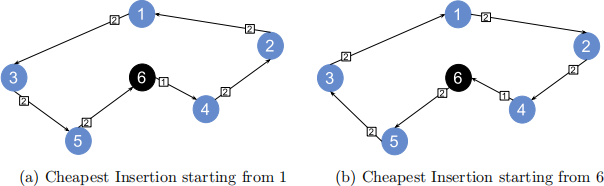
Figure 1: A comparison of the final tour depending where you started the algorithm.
Figure 1(a)’s tour is (1, 3, 5, 6, 4, 2, 1). Figure 1(b)’s tour is (6, 5, 3, 1, 2, 4, 6). While the resulting cost of the tour is the same and looks like it has been reversed, the tour is different. With a larger set of vertices, this can change the resulting tour cost and the final tour.
1.1 Terminology
We will call each point on the graph the vertex. There are 6 vertices in Figure 1.
We will call each connection between vertices the edge.
We will call two vertices connected if they have an edge between them.
The sequence of vertices that are visited is called the tour.
A partial tour is a tour that has not yet visited all the vertices.
We will refer to the weights of all the edges added up in the final or partial tour as the tour cost.
We will refer to the number of vertices in a tour or partial tour as the tour length
2 The solutions
2.1 Preparation of Solution
Just like the previous assignment, you are given a file of coordinates.
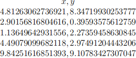
Figure 2: Format of a coord file
Each line is a coordinate for a vertex, with the x and y coordinate being separated by a comma. You will need to convert this into a distance matrix.
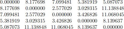
Figure 3: A distance matrix for Figure 2
To convert the coordinates to a distance matrix, you will need make use of the euclidean distance formula.
 (1)
(1)
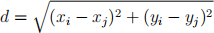
Figure 4: The euclidean distance formula
Where: d is the distance between 2 vertices vi and vj , xi and yi are the coordinates of the vertex vi , and xj and yj are the coordinates of the vertex vj .
2.2 Cheapest Insertion
The cheapest insertion algorithm begins with two connected vertices in a partial tour. Each step, it looks for a vertex that hasn’t been visited and inserts it between two connected vertices in the tour, such that the cost of inserting it between the two connected vertices is minimal.
The steps to Cheapest Insertion can be found on the first assignment brief. Assume that the indices i, j, k etc. are vertex labels, unless stated otherwise. In a tiebreak situation, always pick the lowest index (indices).
2.3 Farthest Insertion
The farthest insertion algorithm begins with two connected vertices in a partial tour. Each step, it checks for the farthest vertex not visited from any vertex within the partial tour, and then inserts it between two connected vertices in the partial tour where the cost of inserting it between the two connected vertices is minimal.
The steps to the farthest insertion algorithm can be found on the first assignment brief. Assume that the indices i, j, k etc. are vertex labels unless stated otherwise. In a tiebreak situation, always pick the lowest index (indices).
2.4 Nearest Addition
The nearest addition algorithm begins with two connected vertices in a partial tour. Each step, it looks for the vertex that’s nearest to a vertex in the partial tour, and adds it to either side of that vertex in the partial tour.
Let G = (V, E) be a graph where V are the vertices, and E : (V × V ) → R + map pairs of vertices to some positive real number.
E.g. E(u, v) = 73.35 where the edge is u → v and the cost of this edge is 73.35.
These graphs are undirected, such that E(v, u) = E(u, v).
Let ⟨v, b, c, d, v⟩ be an example tour representing taking the sequence of edges (v, b),(b, c),(c, d),(d, v).
Suppose we are given adjacency matrix representing G, and a starting vertex v ∈ V .
Steps for implementing the Nearest Addition algorithm go as follows:
1. We start with a tour with only ⟨v⟩. Find the edge that has the smallest E(v, u) cost where u is another vertex in the graph NOT in the tour. From this, generate the tour ⟨v, u, v⟩.
2. Let n be a vertex currently in our stored tour. Find the next edge that has the smallest E(n, x) cost where x is a vertex currently NOT in our tour, and n can be ANY vertex in our tour.
3. At this point, we choose where in our tour we want to place the new vertex x. Depending on the situation, the following restrictions are applied:
• Let an example tour be ⟨v, b, c, d, e, v⟩. Suppose we find a smallest edge (c, x), meaning we will add x to the tour. x can either be added BEFORE or AFTER the position at which c is located, assuming c is NOT AT THE START OR END of the tour.
Possible tours:
⟨v, b, x, c, d, e, v⟩ OR ⟨v, b, c, x, d, e, v⟩
• Let us take the same example tour, but instead suppose (v, x) is the smallest edge. If the vertex being compared is the starting vertex, which indeed should be on both endpoints of the tour, then x can either added AFTER the START vertex, or BEFORE the END vertex.
Possible tours:
⟨v, x, b, c, d, e, v⟩ OR ⟨v, b, c, d, e, x, v⟩
With our choices in mind, take the tour with the LOWEST summed up cost. If the tours happen to have the same summed cost e.g. ⟨v, x, b, c, d, e, v⟩ = ⟨v, b, c, d, e, x, v⟩, then choose the one that would place the new vertex at the leftmost possible location in the tour.
4. Repeat steps 2 and 3 until the whole graph has been processed.
The following is a worked example using Nearest Addition to generate a tour using the pro-vided adjaency matrix, starting from a.
Adjacency Matrix:
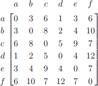
Worked Solution:
Red = vertex already in tour
Blue = vertex being placed in tour
• Current Tour: ⟨a⟩ = 0
Smallest available edge: (a, d) = 1
Add d to tour, put a at end of tour
New Tour: ⟨a, d, a⟩ = 2
• Current Tour: ⟨a, d, a⟩ = 2
Smallest available edge: (d, b) = 2
Tour choices: ⟨a, b, d, a⟩ = 6,⟨a, d, b, a⟩ = 6
Tiebreak: Place b at earliest possible index
New Tour: ⟨a, b, d, a⟩ = 6
• Current Tour: ⟨a, b, d, a⟩ = 6
Smallest available edge: (a, e) = 3
Tour choices: ⟨a, e, b, d, a⟩ = 10,⟨a, b, d, e, a⟩ = 12
New Tour: ⟨a, e, b, d, a⟩ = 10
• Current Tour: ⟨a, e, b, d, a⟩ = 10
Smallest available edge: (d, c) = 5
Tour choices: ⟨a, e, b, c, d, a⟩ = 21,⟨a, e, b, d, c, a⟩ = 20
New Tour: ⟨a, e, b, d, c, a⟩ = 20
• Current Tour: ⟨a, e, b, d, c, a⟩ = 20
Smallest available edge: (a, f) = 6
Tour choices: ⟨a, f, e, b, d, c, a⟩ = 30,⟨a, e, b, d, c, f, a⟩ = 27
Final Tour: ⟨a, e, b, d, c, f, a⟩ = 27
3 Distributed Implementation
You are to implement a distributed implementation using MPI that can find the lowest costing tour for each algorithm. Each algorithm should be run for as many vertices as there are, with each run of an algorithm starting from a different vertex. For example, if there are 4 vertices v0..3, all algorithms should run 4 times each. One run starting from v0, another starting from v1, another from v2, and then finally the last run from v3. The idea is that if you had 4 MPI processes, each process could run 4 instances of Cheapest Insertion (for example) from different starting points. For this example, there would be 12 runs of the algorithms. The Distributed Implementation should run your OpenMP implementations of Cheapest Insertion, Farthest Insertion, and Nearest Addition. In a tiebreak situation, ensure you pick the first lowest costing tour you found.
3.1 Running your programs
Your programs should be able to be run like so:
mpirun −np <p> ./<program >. exe <c o o r d f i l e > <out1> <out2> <out3>
Where p is the number of processes, program is the name of your compiled MPI program, coord file is the name of the coordinate file and out1 is the output file for your lowest costing Cheapest Insertion tour, out2 is the output file for your lowest costing Farthest Insertion tour, and out3 is the output file for your lowest costing Nearest Addition tour.
Therefore, your programs should accept a coordinate file, and 3 output files as arguments. Note that C considers the first argument as the program executable.
Your MPI program should read the data file, run the 3 algorithms, testing for every starting point on each, find the lowest costing tour for each algorithm depending where it started, and write the lowest costing tour of each algorithm to the respective output files.
3.2 Provided Code
You are provided with code that can read the coordinate input from a file, and write the final tour to a file. This is located in the file coordReader.c. You will need to include this file in your compiler command. Declare the functions at the top of your main file, and don’t do #include”coordReader.c” as this has strange behaviour on CodeGrade.
The function readNumOfCoords() takes a filename as a parameter and returns the number of coordinates in the given file as an integer.
The function readCoords() takes the filename and the number of coordinates as parameters, and returns the coordinates from a file and stores it in a two-dimensional array of doubles, where coords[i ][0] is the x coordinate for the ith point, and coords[i ][1] is the y coordinate for the ith point.
The function writeTourToFile() takes a tour, the tour length, and the output filename as parameters, and writes a tour to the given file.
4 Instructions
• Implement an parallel solution for Nearest Addition. Call this file ompnAddition.c
• Implement a serial solution to the Distributed Implementation, that will execute all OpenMP versions of the algorithms and starting points sequentially. Call this main-openmp-only.c
• Implement a parallel solution to the Distributed Implementation that can execute all OpenMP versions of the algorithms and their starting points in parallel. Call this main-mpi.c
• Create a Makefile and call it ”Makefile” which performs as the list states below. With-out the Makefile, your code will not grade on CodeGrade (see more in section 5.1).
– make gomp-only compiles main-openmp-only.c coordReader.c ompcInsertion.c ompfInsertion.c and ompnAddition.c into gomp-only with the GNU compiler (gcc)
– make gcomplete compiles main-mpi.c coordReader.c ompcInsertion.c ompfIn-sertion.c and ompnAddition.c into gcomplete with the GNU MPI compiler (mpicc)
– make iomp-only compiles main-openmp-only.c coordReader.c ompcInsertion.c ompfInsertion.c and ompnAddition.c into iomp-only with the Intel compiler (icc)
– make icomplete compiles main-mpi.c coordReader.c ompcInsertion.c ompfInser-tion.c and ompnAddition.c into icomplete with the Intel MPI compiler (mpiicc)
• Test each of your parallel solutions using 1, 2, 4, 8, 16, and 32 OpenMP threads with just one MPI process, recording the time it takes to solve each process. Record the start time after you read from the coordinates file, and the end time before you write to the output file. Do all testing with the large data file.
• Using the fastest number of threads, test with 1, 2, 4, 8, 16, and 32 MPI Processes. (Note that to run 32 MPI Processes on just the course node alone, you will need to run with 1 OpenMP thread. To see how you can request more nodes for running, look at the section 5.2)
• Plot a speedup plot for the number of threads using 1 MPI process to solve your whole program.
• Plot a strong scaling plot for the number of MPI processes you use. Make sure you explicitly state how many OpenMP threads you used
• Write a report that, for your parallel version of Nearest Addition and your distributed implementation (both serial and parallel), describes your parallelisation strategy.
• In your report, include: the speedup and strong scaling plots, how you conducted each measurement and calculation to plot these, and screenshots of you compiling and running your program. These do not contribute to the page limit
• Your final submission should be uploaded onto CodeGrade. The files you NEED to upload should be:
– Makefile
– coordReader.c
– ompcInsertion.c
– ompfInsertion.c
– ompnAddition.c
– main-openmp-only.c
– main-mpi.c
– report.pdf
5 Hints
You can also parallelise the conversion of the coordinates to the distance matrix.
When declaring arrays, it’s better to use dynamic memory allocation. You can do this by...
int ∗ o n e d a r ra y = ( int ∗) malloc ( numOfElements ∗ s i z e o f ( int ) ) ;
5.1 Makefile
You are instructed to use a MakeFile to compile the code in any way you like. An example of how to use a MakeFile can be used here.
{make command } : { t a r g e t f i l e s }
{compile command}
gc omple te : main−mpi . c coordReader . c om p c I n s e r ti o n . c om p f I n s e r ti o n . c ompnAddition . c
mpicc −fopenmp −s t d=c99 main−mpi . c coordReader . c om p c I n s e r ti o n . c
om p f I n s e r ti o n . c ompnAddition . c −o gc omple te −lm
Now, in the Linux environment, in the same directory as your Makefile, if you type ‘make ci‘, the compile command is automatically executed. It is worth noting, the compile command must be indented. The target files are the files that must be present for the make command to execute. Avoid the -Wall flag when compiling, otherwise if there are any warnings, your code will fail to compile and CodeGrade won’t run your code.
5.2 Running on more than one node
On Barkla, you can use more than just the course node. The reason we tell you to use the course node is because you can execute without having to wait for other users of Barkla (there are a lot). If you want to execute on more than one node, you can use this sbatch command.
sba tch −N <numNodes> −n <numTasks> −c <numCores> −p nodes
By changing the value of -N, we can increase the number of nodes we are using, giving you more resources. On the course partition, we are limited to 1 node with 40 cores. If you wanted to run 32 MPI processes with 32 OpenMP threads, you would need 1024 cores meaning you should request 32 nodes. Ensure you use -p nodes otherwise you will request 32 nodes within the course partition, for which there is only one node, and it will be left in a ”pending” state. Note that you may have to wait several hours (or days/weeks) for your job to have the resources to run, meaning that if you have left the assignment to the last minute, or the job still hasn’t run, test up to 32 MPI processes with just 1 OpenMP thread on the course partition. You can’t actually request 32 nodes on Barkla, but you can do 16.
5.3 Contiguous Memory
With MPI Collective communications, they can only distribute the memory if it is contiguous (if the memory locations are right next to each other). When trying to pass any array that isn’t one-dimensional, there is no guarantee on contiguity, and so MPI will have a problem distributing the array to other processes. To avoid this, you can set up an array as a one-dimensional array, and then reshape it using the following code.
double (∗2 D Array ) [ num] = (double ( ∗ ) [ num ] ) 1 D ar ray ;
Assuming 1D array is an array with num * num elements, this piece of code reshapes a one-dimensional array into a two-dimensional array. So whereas 1D array can be accessed by doing 1D array[i], you can access 2D array by 2D array[i][j]. Note that they share the same memory location, but the compiler will interpret access to memory differently, so any change made to 2D array will also affect 1D array and vice versa.
6 Marking scheme
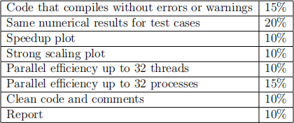
Table 1: Marking scheme
The purpose of this assessment is to develop your skills in analysing numerical programs and developing parallel programs using OpenMP and MPI. This assessment contributes to 35% of this modules grade. The scores from the above marking scheme will be scaled down to reflect that. Your work will be submitted to automatic plagiarism/collusion detection systems, and those exceeding a threshold will be reported to the Academic Integrity Officer for investigation regarding adhesion to the university’s policy https://www.liverpool.ac.uk/media/liva cuk/tqsd/code-of-practice-on-assessment/appendix_L_cop_assess.pdf.
2024-01-04