340        MODEL BUILDING IN MATHEMATICAL PROGRAMMING

Up to six planes can be flown:

n ≤ 6.

13.24.3 Objective

Maximize

(measuring in £1000) where Qi is the probability of scenario i.

This model has 1200 constraints, one bound and 982 variables, of which 117 are 0–1 integer and one general integer.

In defining the data, it is desirable that the demands in the scenarios cover the extremes as well as the most likely cases. The recommended sales will not exceed those of the most extreme scenario in the solution to this model. In this example, it can be seen that final demands (known with hindsight) exceed those of all scenarios in a few cases. As a result, the solution will not result in sales to meet all of these demands.

Models for subsequent weeks (with recourse) are obtained from this model by fixing prices and sales for weeks that have elapsed.

13.25 Car rental 1

We model this problem as a deterministic linear programme. There would be advantage to be gained from modelling it as a stochastic programme. In order to do this, we would need to obtain data to quantify the uncertain demand.

13.25.1 Indices

i ,j = Glasgow, Manchester, Birmingham, Plymouth

t = Monday, Tuesday, Wednesday, Thursday, Friday, Saturday k = 1, 2, 3 (days hired)

Although this is a ‘dynamic’ problem, we seek a steady-state solution and can  therefore regard the set of days as ‘circular’, that is, Monday of a week ‘follows’ after the subsequent Saturday; that is, if t = Monday then t − 1 = Saturday.

13.25.2 Given data

D it = estimated rental demand at depoti on day t as given in Table 12.19

Pij = proportion of cars rented at depot i tobe returned to depot j as given in Table 12.21

Cij = cost of transfer of a car from depot i to depot j as given in Table 12.22

Q k = proportion of cars hired fork days

Ri = repair capacity of depot i

RCAk = rental cost fork days with return to same depot as given in Table 12.23

RCBk = rental cost fork days with return to another depot as given in Table 12.23

RCC    = rental cost for Saturday with return to same depot on Monday

RCD    = rental cost for Saturday with return to another depot on Monday CSk = marginal cost to company of k day hire of a car for all i , t

13.25.3 Variables

n = total number of cars owned

nuit = number of undamaged cars at depot i at the beginning of day t for all i , t

nd it = number of damaged cars at depot i at the beginning of day t for all i , t tr it = number of cars rented out from depot i at beginning of day t for all i , t eu it = undamaged cars left at depot i during day t for all i , t

edit = damaged cars left at depot i at the beginning of day t for all i , t

tuijt = number of undamaged cars at depot i at the beginning of day t , to be transferred to depot j for all i ,j , t

tdijt = number of damaged cars at depot i at the beginning of day t , transferred to depot t for all i ,j , t

rp it = number of damaged cars to be repaired at depoti on day for all i , t

13.25.4 Constraints

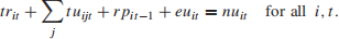
Total number of undamaged cars into depot i on day t

Total number of damaged cars into depot i on day t

Total number of undamaged cars out of depot i on day t

Total number of damaged cars out of depot i on day t

Repair capacity of depot i on all days

rp it ≤ Ri     for all  i,t.

Demand at depot i on day t

tr it ≤ Dit for all  i,t.

Total number of cars equals number hired out from all depots on Monday for 3 days, plus those on Tuesday for 2 or 3 days, plus all damaged and undamaged cars in depots at the beginning of Wednesday.

13.25.5 Objective

Note that £10 has been  added to the profit  on  each rented  car to reflect the surcharge of £100 charged on the  10% of cars that are returned damaged.

This model has a total of 84 constraints and 337 variables.

It is not necessary to constrain the wijkl to  be non-negative. They can be regarded as ‘free’ variables. Avoiding these two stipulations helps the model to solve more easily.

13.26 Car rental 2

We introduce the following 0–1 integer variables with the following interpretations: