EXAMPLE 2: Deep Learning with Time Series and Sequences in MATLAB
Hello, dear friend, you can consult us at any time if you have any questions, add WeChat: daixieit
EXAMPLE 2:
Deep Learning with Time Series and Sequences in MATLAB
Long Short-Term Memory (LSTM) Networks
This lab explains how to work with sequence and time series data for classification and regression tasks using long short-term memory (LSTM) networks.
An LSTM network is a type of recurrent neural network (RNN) that can learn long-term dependencies between time steps of sequence data.
A long short-term memory network is a type of recurrent neural network (RNN). LSTMs excel in learning, processing, and classifying sequential data. Common areas of application include sentiment analysis, language modelling, speech recognition, and video analysis.
The most popular way to train an RNN is by backpropagation through time. However, the problem of the vanishing gradients often causes the parameters to capture short-term dependencies while the information from earlier time steps decays. The reverse issue, exploding gradients, may also occur, causing the error to grow drastically with each time step.
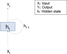
Recurrent neural network.
Long short-term memory networks aim to overcome the issue of the vanishing gradients by using the gates to selectively retain information that is relevant and forget information that is not relevant. Lower sensitivity to the time gap makes LSTM networks better for analysis of sequential data than simple RNNs.
The architecture for an LSTM block is shown below. An LSTM block typically has a memory cell, input gate, output gate, and a forget gate in addition to the hidden state in traditional RNNs.
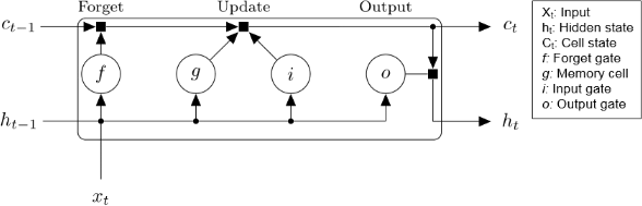
Long Short-Term Memory block.
The weights and biases to the input gate control the extent to which a new value flows into the cell. Similarly, the weights and biases to the forget gate and output gate control the extent to which a value remains in the cell and the extent to which the value in the cell is used to compute the output activation of the LSTM block, respectively.
The core components of an LSTM network are a sequence input layer and an LSTM layer. A sequence input layer inputs sequence or time series data into the network. An LSTM layer learns long-term dependencies between time steps of sequence data.
This diagram illustrates the architecture of a simple LSTM network for classification. The network starts with a sequence input layer followed by an LSTM layer. To predict class labels, the network ends with a fully connected layer, a softmax layer, and a classification output layer.

This diagram illustrates the architecture of a simple LSTM network for regression. The network starts with a sequence input layer followed by an LSTM layer. The network ends with a fully connected layer and a regression output layer.

Objectives
· Create and train networks using Matlab Deep Learning Toolbox for time series classification, regression, and forecasting tasks.
· Train long short-term memory (LSTM) networks for sequence-to-one or sequence-to-label classification and regression problems.
Instructions
Example 1. Classifying speakers by processing spoken Japanese.
You can find this example following this link:
https://uk.mathworks.com/help/deeplearning/ug/classify-sequence-data-using-lstm-networks.html
This example uses the Japanese Vowels data set as described in [1] and [2]. This example trains an LSTM network to recognize the speaker given time series data representing two Japanese vowels spoken in succession. The training data contains time series data for nine speakers. Each sequence has 12 features and varies in length. The data set contains 270 training observations and 370 test observations.
1. Install Deep Learning Matlab Toolbox on your computer if it is not installed yet.
2. Start Matlab.
3. Load the Japanese Vowels training data. XTrain is a cell array containing 270 sequences of dimension 12 of varying length. Y is a categorical vector of labels "1","2",...,"9", which correspond to the nine speakers. The entries in XTrain are matrices with 12 rows (one row for each feature) and varying number of columns (one column for each time step). The 12 features are possibly Mel-Cepstrum coefficients, which represent the total energy in certain frequency bands.
[XTrain,YTrain] = japaneseVowelsTrainData;
XTrain(1:5)
Expected output:
ans=5×1 cell array
{12×20 double}
{12×26 double}
{12×22 double}
{12×20 double}
{12×21 double}
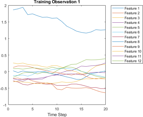
4. Visualize the first time series in a plot. Each line in the diagram corresponds to a feature which value (plotted along y-axis) is changing over time (plotted along x-axis).
figure
plot(XTrain{1}')
xlabel("Time Step")
title("Training Observation 1")
numFeatures = size(XTrain{1},1);
legend("Feature " + string(1:numFeatures),'Location','northeastoutside')
Expected output:
5. Prepare Data for Padding
During training, by default, the software splits the training data into mini-batches and pads the sequences so that they have the same length. Too much padding can have a negative impact on the network performance.
To prevent the training process from adding too much padding, you can sort the training data by sequence length, and choose a mini-batch size so that sequences in a mini-batch have a similar length. The following figure shows the effect of padding sequences before and after sorting data.

a. Get the sequence lengths for each observation.
numObservations = numel(XTrain);
for i=1:numObservations
sequence = XTrain{i};
sequenceLengths(i) = size(sequence,2);
end
b. Sort the data by sequence length.
[sequenceLengths,idx] = sort(sequenceLengths);
XTrain = XTrain(idx);
YTrain = YTrain(idx);
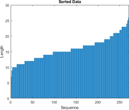
c. View the sorted sequence lengths in a bar chart.
figure
bar(sequenceLengths)
ylim([0 30])
xlabel("Sequence")
ylabel("Length")
title("Sorted Data")
Expected output:
d. Choose a mini-batch size of 27 to divide the training data evenly and reduce the amount of padding in the mini-batches. The following figure illustrates the padding added to the sequences.
miniBatchSize = 27;
6. Define LSTM Network Architecture
Define the LSTM network architecture. Specify the input size to be sequences of size 12 (the dimension of the input data). Specify a bidirectional LSTM layer with 100 hidden units, and output the last element of the sequence. Finally, specify nine classes by including a fully connected layer of size 9, followed by a softmax layer and a classification layer.
If you have access to full sequences at prediction time, then you can use a bidirectional LSTM layer in your network. A bidirectional LSTM layer learns from the full sequence at each time step. If you do not have access to the full sequence at prediction time, for example, if you are forecasting values or predicting one time step at a time, then use an LSTM layer instead.
inputSize = 12;
numHiddenUnits = 100;
numClasses = 9;
layers = [ ...
sequenceInputLayer(inputSize)
bilstmLayer(numHiddenUnits,'OutputMode','last')
fullyConnectedLayer(numClasses)
softmaxLayer
classificationLayer]
7. Specify the training options.
Specify the solver to be 'adam', the gradient threshold to be 1, and the maximum number of epochs to be 100. To reduce the amount of padding in the mini-batches, choose a mini-batch size of 27. To pad the data to have the same length as the longest sequences, specify the sequence length to be 'longest'. To ensure that the data remains sorted by sequence length, specify to never shuffle the data.
Since the mini-batches are small with short sequences, training is better suited for the CPU. Specify 'ExecutionEnvironment' to be 'cpu'. To train on a GPU, if available, set 'ExecutionEnvironment' to 'auto' (this is the default value).
maxEpochs = 100;
miniBatchSize = 27;
options = trainingOptions('adam', ...
'ExecutionEnvironment','cpu', ...
'GradientThreshold',1, ...
'MaxEpochs',maxEpochs, ...
'MiniBatchSize',miniBatchSize, ...
'SequenceLength','longest', ...
'Shuffle','never', ...
'Verbose',0, ...
'Plots','training-progress');
8. Train LSTM Network
net = trainNetwork(XTrain,YTrain,layers,options);
9. Test LSTM Network
Load the test set and classify the sequences into speakers.
Load the Japanese Vowels test data. XTest is a cell array containing 370 sequences of dimension 12 of varying length. YTest is a categorical vector of labels "1","2",..."9", which correspond to the nine speakers.
[XTest,YTest] = japaneseVowelsTestData;
XTest(1:3)
The LSTM network net was trained using mini-batches of sequences of similar length. Ensure that the test data is organized in the same way. Sort the test data by sequence length.
numObservationsTest = numel(XTest);
for i=1:numObservationsTest
sequence = XTest{i};
sequenceLengthsTest(i) = size(sequence,2);
end
[sequenceLengthsTest,idx] = sort(sequenceLengthsTest);
XTest = XTest(idx);
YTest = YTest(idx);
Classify the test data. To reduce the amount of padding introduced by the classification process, set the mini-batch size to 27. To apply the same padding as the training data, specify the sequence length to be 'longest'.
miniBatchSize = 27;
YPred = classify(net,XTest, ...
'MiniBatchSize',miniBatchSize, ...
'SequenceLength','longest');
Calculate the classification accuracy of the predictions.
acc = sum(YPred == YTest)./numel(YTest)
References
[1] M. Kudo, J. Toyama, and M. Shimbo. "Multidimensional Curve Classification Using Passing-Through Regions." Pattern Recognition Letters. Vol. 20, No. 11–13, pages 1103–1111.
[2] UCI Machine Learning Repository: Japanese Vowels Dataset. https://archive.ics.uci.edu/ml/datasets/Japanese+Vowels
Example 2. Sequence-to-Sequence Regression Using Deep Learning
You can find this example following this link:
This example shows how to predict the remaining useful life (RUL) of engines by using deep learning. To train a deep neural network to predict numeric values from time series or sequence data, you can use a long short-term memory (LSTM) network.
This example uses the Turbofan Engine Degradation Simulation Data Set as described in [1]. The example trains an LSTM network to predict the remaining useful life of an engine (predictive maintenance), measured in cycles, given time series data representing various sensors in the engine. The training data contains simulated time series data for 100 engines. Each sequence varies in length and corresponds to a full run to failure (RTF) instance. The test data contains 100 partial sequences and corresponding values of the remaining useful life at the end of each sequence.
The data set contains 100 training observations and 100 test observations.
1. Download the Turbofan Engine Degradation Simulation Data Set from https://ti.arc.nasa.gov/tech/dash/groups/pcoe/prognostic-data-repository/ [2].
Each time series of the Turbofan Engine Degradation Simulation data set represents a different engine. Each engine starts with unknown degrees of initial wear and manufacturing variation. The engine is operating normally at the start of each time series and develops a fault at some point during the series. In the training set, the fault grows in magnitude until system failure.
The data contains a ZIP-compressed text files with 26 columns of numbers, separated by spaces. Each row is a snapshot of data taken during a single operational cycle, and each column is a different variable. The columns correspond to the following:
Column 1 – Unit number
Column 2 – Time in cycles
Columns 3–5 – Operational settings
Columns 6–26 – Sensor measurements 1–21
Create a directory to store the Turbofan Engine Degradation Simulation data set.
dataFolder = fullfile(tempdir,"turbofan");
if ~exist(dataFolder,'dir')
mkdir(dataFolder);
end
2. Unzip the data from the file CMAPSSData.zip.
filename = "CMAPSSData.zip";
unzip(filename,dataFolder)
3. Prepare Training Data
Load the data using the function processTurboFanDataTrain attached to this example. The function processTurboFanDataTrain extracts the data from filenamePredictors and returns the cell arrays XTrain and YTrain, which contain the training predictor and response sequences.
filenamePredictors = fullfile(dataFolder,"train_FD001.txt");
[XTrain,YTrain] = processTurboFanDataTrain(filenamePredictors);
Features that remain constant for all time steps can negatively impact the training. Find the rows of data that have the same minimum and maximum values, and remove the rows.
m = min([XTrain{:}],[],2);
M = max([XTrain{:}],[],2);
idxConstant = M == m;
for i = 1:numel(XTrain)
XTrain{i}(idxConstant,:) = [];
end
View the number of remaining features in the sequences.
numFeatures = size(XTrain{1},1)
Normalize the training predictors to have zero mean and unit variance. To calculate the mean and standard deviation over all observations, concatenate the sequence data horizontally.
mu = mean([XTrain{:}],2);
sig = std([XTrain{:}],0,2);
for i = 1:numel(XTrain)
XTrain{i} = (XTrain{i} - mu) ./ sig;
end
To learn more from the sequence data when the engines are close to failing, clip the responses at the threshold 150. This makes the network treat instances with higher RUL values as equal.
thr = 150;
for i = 1:numel(YTrain)
YTrain{i}(YTrain{i} > thr) = thr;
end
This figure shows the first observation and the corresponding clipped response.
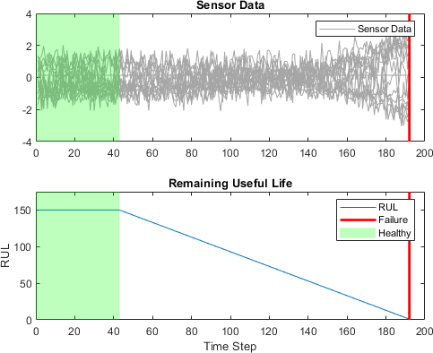
Prepare Data for Padding
To minimize the amount of padding added to the mini-batches, sort the training data by sequence length. Then, choose a mini-batch size which divides the training data evenly and reduces the amount of padding in the mini-batches.
Sort the training data by sequence length.
for i=1:numel(XTrain)
sequence = XTrain{i};
sequenceLengths(i) = size(sequence,2);
end
[sequenceLengths,idx] = sort(sequenceLengths,'descend');
XTrain = XTrain(idx);
YTrain = YTrain(idx);
Choose a mini-batch size which divides the training data evenly and reduces the amount of padding in the mini-batches. Specify a mini-batch size of 20.
miniBatchSize = 20;
4. Define Network Architecture
Define the network architecture. Create an LSTM network that consists of an LSTM layer with 200 hidden units, followed by a fully connected layer of size 50 and a dropout layer with dropout probability 0.5.
numResponses = size(YTrain{1},1);
numHiddenUnits = 200;
layers = [ ...
sequenceInputLayer(numFeatures)
lstmLayer(numHiddenUnits,'OutputMode','sequence')
fullyConnectedLayer(50)
dropoutLayer(0.5)
fullyConnectedLayer(numResponses)
regressionLayer];
Specify the training options. Train for 60 epochs with mini-batches of size 20 using the solver 'adam'. Specify the learning rate 0.01. To prevent the gradients from exploding, set the gradient threshold to 1. To keep the sequences sorted by length, set 'Shuffle' to 'never'.
maxEpochs = 60;
miniBatchSize = 20;
options = trainingOptions('adam', ...
'MaxEpochs',maxEpochs, ...
'MiniBatchSize',miniBatchSize, ...
'InitialLearnRate',0.01, ...
'GradientThreshold',1, ...
'Shuffle','never', ...
'Plots','training-progress',...
'Verbose',0);
5. Train the Network
net = trainNetwork(XTrain,YTrain,layers,options);
6. Test the Network
Prepare the test data using the function processTurboFanDataTest attached to this example. The function processTurboFanDataTest extracts the data from filenamePredictors and filenameResponses and returns the cell arrays XTest and YTest, which contain the test predictor and response sequences, respectively.
filenamePredictors = fullfile(dataFolder,"test_FD001.txt");
filenameResponses = fullfile(dataFolder,"RUL_FD001.txt");
[XTest,YTest] = processTurboFanDataTest(filenamePredictors,filenameResponses);
Remove features with constant values using idxConstant calculated from the training data. Normalize the test predictors using the same parameters as in the training data. Clip the test responses at the same threshold used for the training data.
for i = 1:numel(XTest)
XTest{i}(idxConstant,:) = [];
XTest{i} = (XTest{i} - mu) ./ sig;
YTest{i}(YTest{i} > thr) = thr;
end
Make predictions on the test data using predict. To prevent the function from adding padding to the data, specify the mini-batch size 1.
YPred = predict(net,XTest,'MiniBatchSize',1);
Visualize some of the predictions in a plot.
idx = randperm(numel(YPred),4);
figure
for i = 1:numel(idx)
subplot(2,2,i)
plot(YTest{idx(i)},'--')
hold on
plot(YPred{idx(i)},'.-')
hold off
ylim([0 thr + 25])
title("Test Observation " + idx(i))
xlabel("Time Step")
ylabel("RUL")
end
legend(["Test Data" "Predicted"],'Location','southeast')
For a given partial sequence, the predicted current RUL is the last element of the predicted sequences. Calculate the root-mean-square error (RMSE) of the predictions, and visualize the prediction error in a histogram.
for i = 1:numel(YTest)
YTestLast(i) = YTest{i}(end);
YPredLast(i) = YPred{i}(end);
end
figure
rmse = sqrt(mean((YPredLast - YTestLast).^2))
histogram(YPredLast - YTestLast)
title("RMSE = " + rmse)
ylabel("Frequency")
xlabel("Error")
References
1. Saxena, Abhinav, Kai Goebel, Don Simon, and Neil Eklund. "Damage propagation modeling for aircraft engine run-to-failure simulation." In Prognostics and Health Management, 2008. PHM 2008. International Conference on, pp. 1-9. IEEE, 2008.
2. Saxena, Abhinav, Kai Goebel. "Turbofan Engine Degradation Simulation Data Set." NASA Ames Prognostics Data Repository https://ti.arc.nasa.gov/tech/dash/groups/pcoe/prognostic-data-repository/, NASA Ames Research Center, Moffett Field, CA
2024-01-03