Decision Trees in sklearn
Hello, dear friend, you can consult us at any time if you have any questions, add WeChat: daixieit
Decision Trees in sklearn
We may use decision trees in both classification and regression problems. Here we will solve a classification problem using a decision tree classifier in detail. We will also talk about solving regression problems using the decision tree regressors.
Suppose we want to classify our databased on the target values using a decision tree. For this section, we will use the diabetes_pima data. Let's load the data in our environment first.
>>> import pandas aspd
>>> data = pd_read.csv('diabetes.csv')
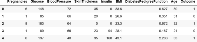
>>> data.head()
>>> data.info()
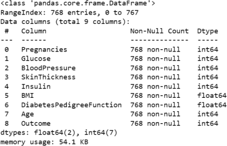
The dataset contains 768 observations (rows) and 8 variables. This dataset is originally from the National Institute of Diabetes and Digestive and Kidney Diseases. The objective of the dataset is to diagnostically predict the onset of diabetes, based on certain diagnostic measurements included in the dataset. Several constraints were placed on the selection of these instances from a larger database. In particular, all patients here are females at least 21 years old of Pima Native American heritage.
variable Information:
• Number of times pregnant.
• Plasma glucose concentration a 2 hours in an oral glucose tolerance test.
• Diastolic blood pressure (mmHg).
• Triceps skinfold thickness (mm).
• 2-Hour serum insulin (mu U/ml).
• Body mass index (weight in kg/(height in m)^2).
• Diabetes pedigree function.
• Age (years).
Class variable (0 or 1). Since the variable 'class' specifies if the banknote is authentic or not that is our target variable. All other variables are our features (predictor variables). Therefore, we have,
>>> features = ['Pregnancies', 'Glucose', 'BloodPressure', 'SkinThickness', 'Insulin', 'BMI', 'DiabetesPedigreeFunction', 'Age']
>>> outcome = 'Outcome'
>>> X = data.loc[:, features].values
>>> y = data.loc[:, outcome].values
Now that we have our features in X and our target in y, we would like to split the training and
testing data sets. Let's import the required package and create X_train, X_test,y_train andy_test, with . Therefore,
>>> from sklearn.model_selection import train_test_split
>>> X_train, X_test,y_train,y_test = train_test_split(X, y, test_size = 0.25, random_state = 1)
We need a Classifier to classify our points. This is done as follows.
>>> from sklearn.tree import DecisionTreeClassifier
>>> classifier = DecisionTreeClassifier(random_state = 1)
Note: The random_state argument in the classifier is used so that the results are the same across different runs.
Now is the time to train our model based on X_train andy_train. This is called fitting and is done using the fit method on the classifier.
>>> classifier.fit(X_train, y_train)
The model (the classifier) has now been trained and has created the tree based on the training data set. The last step for us to is make a prediction based on our X_test. The result of the test will be stored in an array called y_pred. The array y_pred is our predictions on whether or not the banknotes are authentic or not based on features in the X_test. We will later compare y_pred and the true values y_test. Prediction is done using the method predict on the classifier.
>>> y_pred = classifier.predict(X_test)
At this point we are done with the prediction. However, we would like to also evaluate the goodness of our model and algorithm. In order to do that, let's evaluate the results using two methods called the Confusion Matrix and the Classification Report. To get the Confusion Matrix and Classification Report we follow the following.
>>> from sklearn.metrics import classification_report, confusion_matrix
>>> print(confusion_matrix(y_test,y_pred))

>>> print(classification_report(y_test,y_pred))
Arguments of the DecisionTreeClassifier and improving the model
The decision tree classifier has a number of arguments that can be modified. Some include:
• criterion: optional (default=”gini”): by default the value is 'gini', but it can also be changed to 'entropy'. This setting tells the classifier how it should create split points. The two criterion settings are very similar but could in some cases improve results.
• max_depth: optional (default=None): The maximum depth of the tree. The higher value of maximum depth causes overfitting, and a lower value causes underfitting. If max_depth = None, then nodes are expanded until all the leaves contain less than 2. By default max_depth is set to None (if we do not specify it).
Sometimes, we may change arguments of the tree to see if the fit improves. Suppose we are trying to increase the "accuracy" of the model from 72%. We may decide to use a maximum depth of 3 to avoid possible overfitting of the model. Adding that to the classifier we will have,
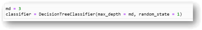
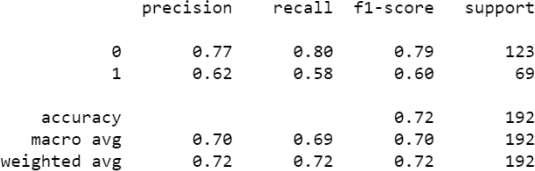
which would result in the following report, which shows an improvement in accuracy from 72% to 78%:
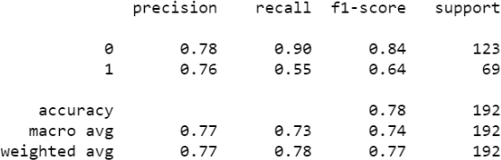
Having deep trees (many layers) may result in overfitting and having a shallow tree may also result in underfitting. There is no set rule for what the perfect depth is. We can try different values of depth and watch for indicators of training and testing accuracy to find out what the best value is. For practice, change the criterion to 'entropy'to see if that improves the model.
To learn about other arguments see this linksklearn.tree.DecisionTreeClassifier — scikit-learn 0.24.2 documentation.
Finding the AUC score
In order to find the AUC score, we will first import the required package.
>>> from sklearn.metrics import roc_auc_score
We will find the AUC score and print it. The result shows a very good AUC score for the model. Apparently the model is able to separate true and false positives from each other very well.
>>> auc = roc_auc_score(y_test,y_pred)
>>> auc
6.692294096854012
Attributes of the Decision Tree Classifier
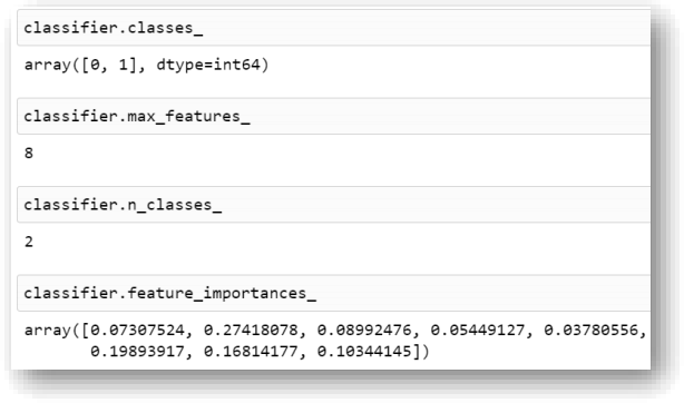
The decision tree classifier model has a number of attributes that we can use once the model is trained. Some of them are listed below.
classes_ : this attribute returns the classes involved in training.
max_features_ : this attribute returns the inferred value of maximum features used.
n_classes_ : this attribute returns the number of classes in the target variable.
feature_importances_ : this attribute returns an array containing feature importance of the
features. The importance of a feature is computed as the (normalized) total reduction of the
criterion brought by that feature. It is also known as the Gini importance. Higher values indicate a higher impact by the feature on the (global) prediction of the model.
Below you can see these attributes for the classifier we trained in this handout.
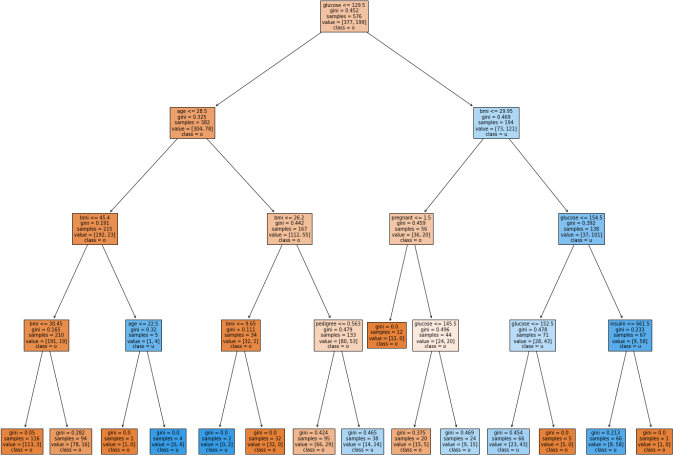
Visualizing Decision Trees
We can visualize decision trees to see the depth of the tree and the number of splits, leaves, etc. The following code block will visualize our decision tree.
>>> from sklearn import tree
>>> import matplotlib.pyplot asplt
>>> plt.figure(figsize=(25,20))
>>> tree.plot_tree(classifier, feature_names=features, class_names=["0"," 1"], filled=True) >>> plt.show()
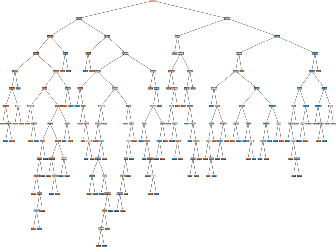
The visualization of the current decision tree in this document is demonstrated below (the first with max_depth = 4 and the second one without specifying that argument).
Decision Tree Regressors
We could also use a decision tree for the purpose of regression. The process would be completely similar to the linear regression with sklearn that wereviewed before. The difference is instead of using LinearRegression() to create the model, we will use a
DecisionTreeRegressor() to create the model. Observe how we can import and use it to create the model.

We can a regression model using this method and the rest of the process is exactly similar to what was discussed in the Linear Regression handout.
Notes:
• Similar to DecisionTreeClassifier(), we can use the max_depth argument in DecisionTreeRegressor() as well.
• Similar to DecisionTreeClassifier(), there are attributes that we can use to get details on the model. Some of these attributes are listed below:
o max_features_ : The inferred value of max_features.
o feature_importances_ : The inferred value of max_features.
After creating a model using DecisionTreeRegressor(), we can use the same evaluation techniques that we used for a Linear Regression model to evaluate the model, i.e., MSE, RMSE, r2 , etc. Obviously, the model being a decision tree, does not have coefficients (unlike a linear regression model).
2024-01-03