For each  model,  report the estimated  parameters, their corresponding t statistic and the coefficient of determination of the model. Provide a plot for each model which demonstrates how it fits the data.

Model Selection

Discuss your findings from the model estimation process. In specific explain the following items

1.   Which coefficients are statistically significant, and which ones are not?

2.    Explain the meaning of the estimated coefficients and whether the estimated sign is expected or not.

3.   Discuss the magnitude of the models’ intercept.

4.   Compare the goodness-of-fit of the models (coefficient of determination).

Select the most suitable model out of the five estimated models. Justify your choice based on the discussed items in this section and the number of independent variables in the model.

Section 2: Development and Application of a Gravity Model

The picturesque Sharington region is a rapidly developing area to the southwest of the major metropolis of Givingly, a city which has similar features to that of Sydney, Australia. Sharington is 50km away from the CBD of Givingly and as a result, the region contains residential, commercial and industrial land uses. Growth and appeal of the area are a result of housing price pressure and improving transport infrastructure which has increased accessibility to and from Sharington.

Sharington  Local  Council  is  preparing  a  transport  master  plan  and  is  seeking  transport planning advice from your consulting firm. Sharington can be separated into 5 zones as shown in Figure 1.

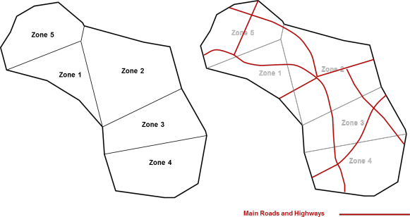
Figure 1: Study area of Sharington Local Council

Intra-zonal travel is present and the geography of the study area has resulted in some zones being adjacent to one another whilst others are separated and connected with the  road network as presented in Figure 1 (note that this represents only main roads and highways). Recently, Sharington conducted traffic surveys during the  morning AM  peak  period. The surveys were  processed  to  form  a  travel  time  matrix  (presented  in  Table  1)  and  a  trip distribution matrix (presented in Table 2) that provides an accurate reflection of the existing travel conditions during the AM peak period. The adjacency and separation of the zones are reflected  in  the  travel  times  and  as  such  the  council  has  urged  your  consulting  firm  to categorise the zones and zone-to-zone travel based on geographical proximity.

Table 1: Observed travel time matrix

Table 2: Observed Trip Distribution Matrix

Answer the following questions:

a)   Based on the information presented in the description, define appropriate travel time intervals for the region and categorise each zone within the region into the defined    travel time intervals. Present your categorisation clearly using a table.

b)  Sharington Local Council has requested for the trip distribution in the study area to be estimated using a gravity model

i.      Calibrate the gravity model for the given existing travel time matrix and observed trip distribution.

ii.      Which zone pairings least match the observed counts? Provide a reason for why these zone pairings differ more than the other zone pairings?

iii.      Estimate the mean absolute error ratio for this model. Provide a comment on the acceptability of the model.

c)   Use the 2025 expected travel time matrix (see Table 3) and the predicted   productions and attractions of Sharington (see Table 4) to estimate the trip distribution in 2025.

i.      Use the calibrated friction factors and socio-economic parameters to apply  the gravity model. Perform row and column factoring to obtain a converged model and present the trip distribution rounded to the nearest integer.

ii.      Describe in 3 dot-points the differences between the existing travel patterns in Sharington and the 2025 travel patterns.

Table 3: 2025 expected travel time matrix

Table 4: Predicted Productions and Attractions of each zone in 2025

Section 3: Introduction to Mode Choice

The introduction of the CBD & South East Light Rail in Sydney will provide an additional mode of travel for commuters between the CBD and UNSW. The state government acknowledge that the success of the light rail introduction will be based on uptake of the service and the following mode choice exercise can be used to discover the potential impacts.

Currently, there are two possible modes to travel to UNSW from the CBD; using a private vehicle (car) or using the bus service. A study into the satisfaction and features of each mode yielded the following calibrated utility function:

Uk = ak 一 0.025xaccess 一 0.032xwait 一 0.015xinvehicle 一 0.001xcost

Where: xaccess= Access and egress time of mode K (minutes)

xwait = Waiting time of mode K (minutes)

xinvehicle = In-vehicle travel time of mode K (minutes)

xcost = monetary cost to travel on a single trip using mode K (cents)

ak = constant

The variable values for the car mode and the bus service are presented in Table 1.

The current demand for travel between the CBD and UNSW is 80,000 trips per day. The expected demand in the future scenario is 100,000 trips per day.

Considering the description, please answer the questions below

a)  What type of utility formulation is used? What is an advantage of using this

formulation and why is it an advantage? What is the significance of the constant ak   in the function?

b)  Apply the logit mode to estimate the existing mode-share between car and bus

(present proportions (rounded to 2 d.p.) and number of trips, rounded to the nearest   integer). What type of logit model was applied? What is the daily revenue that can be generated from the bus service?

Another stated  preference survey conducted by the state government  provided customer expectations of the attributes of the existing modes and the future light rail system. In addition to this, transport planners have determined the cost of using all 3 modes in the future. The forecasted variable values for the three modes are presented in Table 2

c)   Apply the logit mode to estimate the future mode share between the 3 modes

(present proportions (rounded to 2 d.p.) and number of trips, rounded to the nearest   integer). What type of logit model was applied? What is the daily revenue that can be generated from all public transport services?

d)  Will the inclusion of light rail increase fare revenue for the state government? Is fare revenue the only factor to consider when introducing a new mode or any new public transport infrastructure? If not what are other factors transport planners and traffic engineers would consider.

As a means to reduce private vehicle usage in the study corridor, the state government is considering the following proposals.

.     Proposal A: Reduction of parking provision across the corridor, increasing the expected access time to use a car by a further 5 minutes.

o The daily cost of implementing this proposal to the government is estimated to be $10,000.

.     Proposal B: Increasing registration costs of private vehicle owners such that the cost of a trip increases by half of the existing cost.

o The daily cost of implementing this proposal to the government is estimated to be $15,000.