CSE 250a. Assignment 4
Hello, dear friend, you can consult us at any time if you have any questions, add WeChat: daixieit
CSE 250a. Assignment 4
4.1 Maximum likelihood estimation of a multinomial distribution
A 2D-sided die is tossed many times, and the results of each toss are recorded as data. Suppose that in the course of the experiment, the d th side of the die is observed Cd times. For this problem, you should assume that the tosses are identically, independent distributed (i.i.d.) according to the probabilities of the die.
(a) Log-likelihood
Let X ∈ {1, 2, 3, . . . , 2D} denote the outcome of a toss, and let pd = P(X = d) denote the proba-bilities of the die. Express the log-likelihood L = log P(data) of the observed results in terms of the probabilities pd and the counts Cd.
(b) Maximum likelihood estimate
Derive the maximum likelihood estimates of the die’s probabilities pd. Specifically, maximize your expression for the log-likelihood L in part (a) subject to the constraints
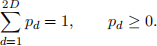
You should use a Lagrange multiplier to enforce the linear equality constraint, but it is sufficient to observe that the resulting solution is nonnegative.
(c) Even versus odd
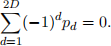
Compute the probability P(X ∈ {2, 4, 6, . . . , 2D}) that the roll of a die is even and also the proba-bility P(X ∈ {1, 3, 5, . . . , 2D − 1}) that the roll of a die is odd. Show that these two probabilities are equal when
(d) Maximum likelihood estimate
Suppose it is known a priori that the probability of an even toss is equal to that of an odd toss. Derive the maximum likelihood estimates of the die’s probabilities pd subject to this additional constraint. Specifically, maximize your expression for the log-likelihood L in part (a) subject to the constraints
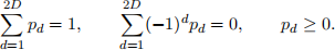
Hint 1: introduce two Lagrange multipliers, one for each linear equality constraint.
Hint 2: it may simplify your final answer to let  denote the sums of even and odd counts.
4.2 Maximum likelihood estimation in belief networks
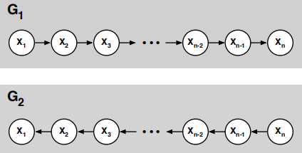
Consider the two DAGs shown below, G1 and G2, over the same nodes {X1, X2, . . . , Xn}, that differ only in the direction of their edges.
Suppose that we have a (fully observed) data set  in which each example provides a complete instantiation of the nodes in these DAGs. Let COUNTi(x) denote the number of examples in which Xi =x, and let COUNTi(x, x′) denote the number of examples in which Xi =x and Xi+1 =x
′.
in which each example provides a complete instantiation of the nodes in these DAGs. Let COUNTi(x) denote the number of examples in which Xi =x, and let COUNTi(x, x′) denote the number of examples in which Xi =x and Xi+1 =x
′.
(a) Express the maximum likelihood estimates for the CPTs in G1 in terms of these counts.
(b) Express the maximum likelihood estimates for the CPTs in G2 in terms of these counts.
(c) Using your answers from parts (a) and (b), show that the maximum likelihood CPTs for G1 and G2 from this data set give rise to the same joint distribution over the nodes {X1, X2, . . . , Xn}.
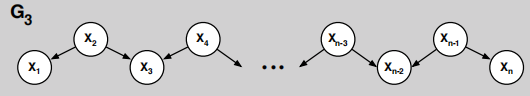
(d) Suppose that some but not all of the edges in these DAGs were reversed, as in the graph G3 shown below. Would the maximum likelihood CPTs for G3 also give rise to the same joint distribution?
(Hint: does G3 imply all the same statements of conditional independence as G1 and G2? Look in particular at nodes X3 and Xn−2.)
4.3 Statistical language modeling
In this problem, you will explore some simple statistical models of English text. Download and examine the data files on Canvas for this assignment. (Start with the hw4_readme.txt file.) These files contain unigram and bigram counts for 500 frequently occurring tokens in English text. These tokens include actual words as well as punctuation symbols and other textual markers. In addition, an “unknown” token is used to represent all words that occur outside this basic vocabulary. For this problem, as usual, you may program in the language of your choice.
(a) Compute the maximum likelihood estimate of the unigram distribution Pu(w) over words w. Print out a table of all the tokens (i.e., words) that start with the letter “M”, along with their numerical unigram probabilities (not counts). (You do not need to print out the unigram probabilities for all 500 tokens.)
(b) Compute the maximum likelihood estimate of the bigram distribution Pb(w ′|w). Print out a table of the ten most likely words to follow the word “THE”, along with their numerical bigram probabilities.
(c) Consider the sentence “The stock market fell by one hundred points last week.” Ignoring punctua-tion, compute and compare the log-likelihoods of this sentence under the unigram and bigram models:
Lu = log [Pu(the) Pu(stock) Pu(market) . . . Pu(points) Pu(last)Pu(week)]
Lb = log [Pb(the|⟨s⟩) Pb(stock|the) Pb(market|stock) . . . Pb(last|points) Pb(week|last)]
In the equation for the bigram log-likelihood, the token ⟨s⟩ is used to mark the beginning of a sentence. Which model yields the highest log-likelihood?
(d) Consider the sentence “The sixteen officials sold fire insurance.” Ignoring punctuation, compute and compare the log-likelihoods of this sentence under the unigram and bigram models:
Lu = log [Pu(the) Pu(sixteen) Pu(officials) . . . Pu(sold) Pu(fire) Pu(insurance)]
Lb = log [Pb(the|⟨s⟩) Pb(sixteen|the) Pb(officials|sixteen) . . . Pb(fire|sold) Pb(insurance|fire)]
Which pairs of adjacent words in this sentence are not observed in the training corpus? What effect does this have on the log-likelihood from the bigram model?
(e) Consider the so-called mixture model that predicts words from a weighted interpolation of the unigram and bigram models:
Pm(w ′|w) = λPu(w ′) + (1 − λ)Pb(w ′|w),
where λ ∈ [0, 1] determines how much weight is attached to each prediction. Under this mixture model, the log-likelihood of the sentence from part (d) is given by:
Lm = log [Pm(the|⟨s⟩) Pm(sixteen|the) Pm(officials|sixteen) . . . Pm(fire|sold) Pm(insurance|fire)].
Compute and plot the value of this log-likelihood Lm as a function of the parameter λ ∈ [0, 1]. From your results, deduce the optimal value of λ to two significant digits.
(f) Submit a printout of your source code for the previous parts of this problem.
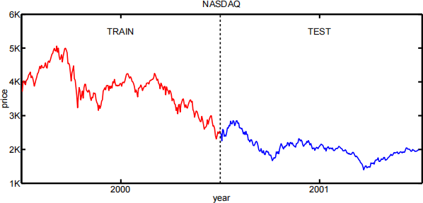
4.4 Stock market prediction
In this problem, you will apply a simple linear model to predicting the stock market. From the course web site, download the files nasdaq00.txt and nasdaq01.txt, which contain the NASDAQ indices at the close of business days in 2000 and 2001.
(a) Linear coefficients
How accurately can the index on one day be predicted by a linear combination of the three preceding indices? Using only data from the year 2000, compute the linear coefficients (a1,a2,a3) that maximize the log-likelihood  , where:

and the sum is over business days in the year 2000 (starting from the fourth day).
(b) Root mean squared prediction error
For the coefficients estimated in part (a), compare the model’s performance (in terms of root mean squared error) on the data from the years 2000 and 2001. (A rhetorical question: does a lower predic-tion error in 2001 indicate that the model worked better that year?)
(c) Source code
Turn in a print-out of your source code. You may program in the language of your choice, and you may solve the required system of linear equations either by hand or by using built-in routines (e.g., in Matlab, NumPy).
2023-12-29