2.   Background

2.1 Model background

The hydrology of the Rio Grande Headwaters in Colorado, USA is snowmelt dominated. It varies considerably from year to year and may very further under a changing climate. One of the tools we use to understand monitor processes in such

an area is a mathematical ('environmental') model describing the main physical processes affecting hydrology in the catchment. Such a model could help understand current behaviour and allow some prediction about possible future  scenarios.

In this part of your assessment you will be using, calibrating and validating such a model that relates temperature and snow cover in the catchment to river flow.

We will use the model to describe the streamflow at the Del Norte measurement station, just on the edge of the catchment.

You will use environmental (temperature) data and snow cover observations to drive the model. You will perform calibration and testing by comparing model output with observed streamflow data.

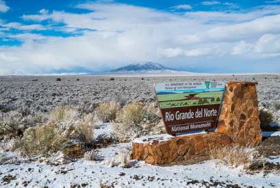
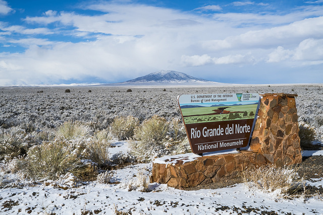
Figure 1.Del Norte station

2.2.Del Norte

Further general information is available from variouswebsites, includingNOAA. You can visualise the site Del Norte 2Ehere. This is the site we will be using for river discharge data.

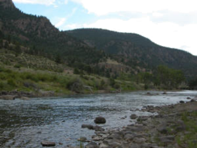
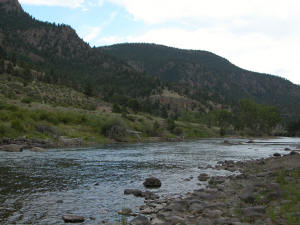
Figure 2.River near Del Norte station

2.3 Model

2.3.1 Model basics

We will build a simple mass balance model that is capable of predicting daily streamflow at some catchment location forgiven temperature and catchment snow cover. This defines the purpose of our model (how we will use it) and describes the model output (daily streamflow QdN [t] at some catchment location) and drivers (temperature T [t] and catchment snow cover p[t]):

We will need 2 dynamic datasets to run the model, given for samples in time t:

.     T [t]: mean temperature (C) at the Del Norte monitoring station for each day of the year

.     p[t]: Catchment snow cover (proportion)

and one dataset to calibrate and test the model, for samples in time:

.     QdN [t]: stream flow data for each in units of megalitres/day (ML/day i.e. units of 1000000 litres a day) at the del Norte monitoring station.

You should already have the datasets T [t] and QdN [t] for the years 2016-2019 inclusive, and will need to make use of the datasets for 2018 and 2019 in this work. In the first part of this submission we will deriving the snow cover data from MODIS satellite data. We will explain this below.

As we have noted, you will be running, calibrating and testing a mass-balancesnowmelt model in the Rio Grande Headwaters in Colorado, USA.  In such a model, we keep track of the mass of some parameter of interest, here the snow water-equivalent (SWE), the amount of water in the snowpack for the catchment. We assume the reservoir of water is    directly proportional to snow cover p[t]at time tso:

SWE[t] = k1 p[t]                                                  (1)

with k1 a constant of proportionality relating to snow depth and density.

In the model, we do not consider mechanisms of when the snow appears or disappears from any location or thinning/thickening of the snowpack. Rather, we use the snow cover as time t, p[t], as a direct surrogate of the SWE at time t.

2.3.2 Water release

We need a mechanism in the model that converts from SWE[t]to flow dQ[t], the water flowing into the system from the snowpack at time t. We can consider this as:

dQ[t] = k2 m[t] SWE[t]

= k1 k2 m[t] p[t]

= k m[t] p[t]                                            (2)

where dQ[t]is the amount of water flowing into the catchment at time t, m[t] is a proportion of the snowpack assumed to melt at time t, and k2 a constant of proportionality relating to the proportion of the SWE that is available to be converted. We combine the constants of proportionality so k=k1  k2.

You can imagine the snow water equivalent SWE[t]as a quantity of snow in a bucket observed at time t, and there being some proportion k2 of this that has the potential to melt and become water dQ[t]. You can think of there being a tap or valve that releases that water into another bucket at time t, with m[t] (between 0 and 1) being a measure of how much that valve is open or closed. The main control on this tap is temperature at time t, T [t]. In the simplest form, this would be a switch, so setting m to 0when flow is off (too cold to melt) and m to 1when flow is on (hot enough to melt). Practically, we model the rate of release of water from the snowpack as a logistic function of temperature:

m[t] = expit([T[t]-T0 ]/xp )                                      (3)

where expit the logistic function that we have previously used in phenology modelling. This is a form of'soft'switch between the two states (still with melting, m=0, and melting m=1). If the temperature is very much less than the threshold T0, it will remain frozen. If it is very much greater than T0, there will bean amount proportionate to SWE[t] flowing into the system on day t.

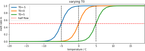
Figure 3. melt rate m[t] for varying value of parameter T0

The parameter, xp (C) increases the slope of the function at T=T0 with increasing xp. So it can be used to modify the 'speed' of action, or ‘sensitivity’ of the soft switch. We will use a default value of xp=1. It is likely to have only a minor impact on the modelling results so we can use this assumed value of the parameter. By keeping this parameter at a fixed value, we can simplify the problem you need to solve to one involving a single parameter to model the water release. We assume that T0 can be calibrated for a given catchment.

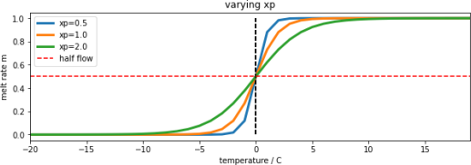
Figure 4. melt rate m[t] for varying value of parameter xp for T0=0

Notice that the threshold temperature T0 is not really the temperature at which melting begins: we can see from above that for xp=1.0, melting occurs at temperatures above around T0-5C. Also, consider that the temperature data we will be using is the temperature at the Del Norte station, and that this is likely some degrees higher than the temperature in  the mountains where the snowmelt will be occurring. For these various reasons, we would not expect T0to be 0C, but somewhat higher, perhaps closer to 10 C.  We should call this parameter a threshold temperature, rather than a ‘melting temperature’. Notice that if we decrease the sensitivity parameter xp, then the range of ‘melting temperatures’ is also reduced, so we might expect T0 to decrease with decreasing xp. So, although changing xp might have only a small impact on the result, it is likely to have a correlation with the parameter T0.

So:

dQ[t] = k p[t] expit((T [t]-T0 )/xp )                              (4)

This is driven by T [t] and p[t] and controlled by parameters T0 and to a lesser extent xp. If we normalise our measures, i.e. dQ[t]/dQmax and QdN [t]/QdNmax, with dQmax and QdNmax, being the maximum values of Q[t] and QdN [t] respectively, then we can compare the quantity of meltwater at time t with the measured flow at the monitoring station.

In the figure below, we see the normalised modelled meltwater dQ[t] (scaled) that corresponds to a T0  of 9 C derived from datasets T [t] and p[t], alongside the normalised measured flow QdN [t] (scaled) at the del Norte station. dQ[t] is remarkably similar to the flow data QdN [t], but much noisier. We also see that it occurs sometime before we see the    water flow at the monitoring station. The reason for this is that there is a 'network delay' between the melt happening in the snowpack and it reaching the monitoring station. This final component of our model is a network response function   (NRF) that models this delay in the routing of the meltwater.

Figure 5. Available water dQ[t] for T0=9 C (green) plotted alongside measured flow (black) and driving data

2.3.3 Flow delay to the measuring stations

To be able to generate our desired model output, we now have to consider how this reservoir of water is transported to predict daily streamflow at some catchment measurement location. We do this using the concept of a Network Response Function (NRF). In this sub-model, we assume that the flow from out reservoir dQ[t]to the catchment measurement

location can be characterised as a decay function after time t=0. So, some proportion of the water released is

immediately transported to the station, and a lesser amount reaches the next day, and less the next day and soon. So, if we put a pulse of water into the system we would measure a simple decay function. This pulse response is the NRF.

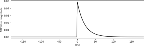
Figure 6. Network Response Function (NRF) as a function of time to f=20 days

The NRF is effectively a one-sided smoothing filter. It imparts a delay on the signal dQ[t] and smooths it. We can use a function such as a one-sided Laplace distribution, a one-sided exponential parameterised by a rate of decay value f (days) to model the probability of water reaching the monitoring station at time t.

Q’dN [t] = dQ[t] * L1 (t/f)                                       (5)

Where Q’dN [t] is the modelled flow (we use ’for modelled flow here) output at the del Norte station, * is the

convolution operator,dQ[t]is the snowmelt entering the reservoir at time t,  and  L1 (t/f) is the NRF response, a one-sided Laplace (exponential) distribution:

L1 (x) = exp[-x]/N | x >= 0                                     (6)

0         |

with the normalisation factor:

N = Σ  L1 (x)

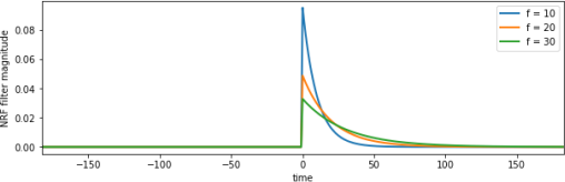
Figure 7. Network Response Function (NRF) as a function of time for varying f

You can think of this model as allowing the meltwater that becomes available at time t, dQ[t], to be spread out over time when it reaches the monitoring station. So, in figure 7 for f=10, around 0.09 of the meltwater goes immediately to the monitoring station, then less than that the next day, and soon, until almost all of the water has reached the station after around 40 days.  The ‘spread’ of this then is controlled by the parameter f. Iff is increased to 20,  only 0.05 of the water goes directly to the station, and it is spread out over a longer time period.  So, f is characteristic of the catchment physical properties and the location of the snow sources relative to the monitoring station. We assume it to be a constant here, something that can be calibrated for the catchment and station.

2.3.4 Model

If, for the moment, we ignore the parameter xp, then we can illustrate out model as in the figure below:

Figure 8. Model description

The complete model has three parameters that control model behaviour:

.     the threshold temperature T0 (C);

.     the delay parameter f (days) of the Network Response Function (NRF)

.     the temperature sensitivity parameter xp  (C)

Summary:

In this coursework,  you must estimate the two main parameters (T0 and f) for the catchment in a model calibration stage using data from 2018, and then validate the calibrated model against independent data from the year 2019. This requires you to compare the predicted station streamflow Q’dN [t]with measured values QdN [t] in some optimisation routine using a model driven by daily temperature T[t] and snow cover p[t]. You will first need to derive the estimate of  snow cover for the two years.

You can find code implementing and running the model innotebooks/066_Part2_code.ipynbin the notes.

warp_args = {

'dstNodata'

'format'

'cropToCutline' 'cutlineWhere'

'cutlineDSName'

}

: 255,

: 'MEM',

: True,

: f"HUC=13010001",

: 'data/Hydrologic_Units/HUC_Polygons.shp'

You can the use a high-level function such as modisAnnual as previously in the notes to gather the dataset for the two years of  interest, but that if you do, the marks you get for that part of the code development will be limited to a pass grade. You can get more marks by developing, documenting and commenting your own codes for the MODIS processing.