Physics 307 Project 8
Hello, dear friend, you can consult us at any time if you have any questions, add WeChat: daixieit
Physics 307 Project 8
First two parts due Friday, December 1; the final part is due on Friday, December 8
In this project you will study the properties of your vibrating string. You have nothing (much) to code this time, but you have quite a few things to simulate, study, and discuss.
A common exercise in physics is to study a simplified model of a vibrating string where we assume that the amplitude is small and the tension is large; this gives rise to the familiar behavior we will discuss in class. For your project, you will examine this behavior, and discover the limits of its validity.
As a reminder, some properties of the vibrating string in this limit:
• Oscillations are a superposition of normal modes:  , where L is the stretched length
• Waves propagate along the string at a rate 
• The n’th normal mode has a wavelength  , giving it a period
• These properties don’t depend on the amplitude, in the limit of small amplitude.
Part 1: Verifying your code and testing the ideal behavior (due Friday, December 1)
1. Modify your initial conditions to simulate any normal mode of your choice. Then modify your code to print out the period of your string; you can determine the half-period by looking for points at which the velocity at an antinode changes sign. (“If it was going up before, and now it’s going down, then we’re at a half-period” – you did a similar thing for the pendulum.) Note that this is only valid if you have behavior that’s relatively close to the vibration of a normal mode; otherwise, the idea of “period” is more complicated.
2. Recall that our goal was to simulate a vibrating string using only N and the macro-scopic quantities T, α, µ, and L0. All microscopic quantities (the node mass m, the individual spring constant k ′ , and the equilibrium radius r0 should be determined from these.
You need to verify that you are correctly implementing the relationship between the macroscopic quantities and the microscopic quantities. You can do this by simulating something well-behaved and verifying that the period doesn’t depend on N. Use enough tension to stretch your string to 1.3-1.5× its starting length, and then simulate the fundamental mode (n = 1) at a small amplitude. Verify that the period doesn’t depend (much) on N. This is one check that everything is working properly.
3. Now, adjust the tension, linear density, unstretched length, and verify that the period has the expected dependence on them. Remember, this expected dependence is only valid in the “well-behaved” realm, where T is large and the amplitude is small.
IMPORTANT NOTE: The linear mass density µ that appears in the expression for the wave speed, and the quantity L that you use to compute the wave speed, are the values after you stretch the string. You may handle this in any way you choose; one is to compute a stretched density µ ′ after you determine the stretch length that gives the specified tension.
Part 2: Superpositions of normal modes (also due Tuesday, November 27 as well)
As you know, the vibrations of a string (in the ideal case) can be characterized by a superposition of normal modes.
4. You can also excite the string in more physical ways and study its behavior. Modify your initial conditions so that you give the string a Gaussian “bump” in either velocity or position in the beginning. Specifically,
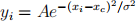
where xc is the center of the bump, and σ is its width; A is an amplitude. (Make sure xc >> σ, or you’ll be moving one of the endpoints significantly.) You will probably want to use a small amplitude to avoid blatantly nonlinear behavior.
If your small amplitude makes the vibrations too small to see easily, you can always multiply the y-coordinates by some factor when you display them, just to exaggerate the motions to make them more visible.
This lets you excite the string with either a “soft” impulse, like a fingertip, or a “sharp” impulse, like a guitar pick. You can also do this at different points on the string, from the center to near the edge.
Try different sorts of excitation and qualitatively examine the character of the vibra-tions produced. Mathematically, you would use a Fourier transform to determine the amplitudes of the different normal modes, but you don’t need to do that here; it’s enough to look at the overall character: “little fast wiggles” means that there is lots of energy in the higher normal modes, while “slow big waves” means that there is lots of energy in the lower modes.
5. Acoustically, an excitation that involves mostly lower normal modes sounds “darker” or more “mellow”; an excitation that involves significant energy in the higher normal modes sounds “bright” or “tinny”. Consider the difference between exciting a guitar string with a pick (which applies a force to a very small region of the string) and a finger (which applies a force to a larger region of the string). Simulate something corresponding to each of these and look at the oscillation of your string. Does the observed behavior match the expected sound?
Part 3: Testing the nonlinear behavior you can’t do with pen and paper (due Friday, December 8)
Note: This part may be modified in the next few weeks.
6. Now we’re going to deviate from the limit of small amplitude (i.e. “what you learned in pencil-and-paper physics class”) and look at the non-ideal behavior. Simulate a few different normal modes at a range of amplitudes (ranging up to A ≃ L), and also vary the tension. Discuss the validity of the “normal mode” idea outside of the limit of small amplitude: does your simulation now exhibit independent normal modes, each with a definite frequency?
7. Calculate the fractional difference between your measured period and the analytic period for different values for the amplitude, going roughly from small A to A = 0.4L. (Include enough points that the character is clear). As a reminder, the analytic value for the period, correct for small amplitude, is
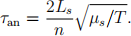
Thus the fractional difference ∆τ can be defined as

where τnum is the numeric period you measure with your program. This should give you a ∆τ value close to zero for small amplitude. (For small amplitudes, the difference will be dominated by modeling error and numerical error in your simulation, rather than by any amplitude effects. You will want to minimize these as best you can.)
Now, since both ∆τ and A are small for small amplitude, you can plot your data on a log-log plot to really see what is going on. Do so; how does ∆τ depend on amplitude? Comment on similarities and differences between this project and the pendulum project.
Gather two sets of data: one for the n = 1 and one for the n = 4 mode. Plot them on top of each other, and determine which normal mode is most subject to large-amplitude effects.
8. If a musician excites a string when playing an instrument, the string’s amplitude will decay from its initial value down to zero as the oscillations are slowly damped, so each note will cover a range of amplitudes. Given that a deviation in frequency of 5% is “grossly out of tune” and a deviation of 1% is audibly out of tune, speculate on the impact of the amplitude-frequency connection on music.
2023-12-26