Aerospace Dynamics – Vibrations & Aeroelasticity
Hello, dear friend, you can consult us at any time if you have any questions, add WeChat: daixieit
Aerospace Dynamics - Vibrations & Aeroelasticity
December 2023 assessment
Academic year 2023-2024 coursework specification
Application of a TVA in an aircraft
Students must submit their own individual and independent work. All submitted reports will be checked against plagiarism in all their aspects.
Coursework description
This Vibrations theme coursework constitutes 50% of the final mark in the unit. The coursework centres on an application example of an aircraft which suffers from excessive vibrations in one of its parts. The coursework is divided into 5 tasks. Each task contributes 20% to the overall mark for the coursework. Further marking information is provided in section Marking (page 3).
Each task must be answered on a single page in the final individual report. The final report will consist of a single title page (which should include all relevant ID details, in particular name and UoB username) and five additional pages covering the technical tasks. This assessment closes a 10cp component of Aerospace Dynamics. With this credit weight, the component corresponds to approximately 100 hours of study. Within this context and assuming the nominal engagement with the taught content, the coursework is designed to be completed during five days of individual work.
Those students who wish to start with tasks 1, 2 and 3 are recommended to read Appendix first to appreciate the context and to familiarise with the provided software tool.
Contents
Coursework specification and guidance 3
Task 1: Single degree-of-freedom analysis (20% of 100%) 4
Task 2: General two degree-of-freedom analysis (20% of 100%) 5
Task 3: Tuned Vibration Absorber (20% of 100%) 6
Task 4: Equations of motion for 2 DOF system and eigenvalue problem (20% of 100%) 7
Task 5: Transient aeroelastic simulation of 2 DOF system (20% of 100%) 8
AfCh … Amplitude-frequency characteristics
|
DOF |
… degree of freedom |
|
EoM |
… Equation of Motion |
|
FRF |
… Frequency Response Function |
|
ODE |
… ordinary differential equation |
abc … typed Matlab text
Coursework specification and guidance
Each task is specified in terms of its technical objective and the expected delivery format. All tasks should have page layout consistent with the following example. Each task specification offers further detail on what are the recommended proportions between the compulsory Results and Discussion sections.

Writing recommendations and page formatting:
• A4 page size, all page margins minimum 2 cm and maximum 2.5 cm wide.
• Font size 10pt or 11pt, single line spacing.
• Use figure captions, include and use SI units, label or annotate where appropriate, use legends.
• Describe all figures and tables using a brief description.
• Use variety of line styles, data markers, choose suitable font size, ensure clear visibility.
• Use formal language, avoid the use of the first person in discussions or elsewhere.
• Preferably avoid the use of photographed hand-drawn sketches.
• In discussions, focus on covering the required discussion topics.
• Preferably avoid trivial, obvious, repetitive, or irrelevant discussion points.
• “briefly”, “brief statement”, “short paragraph”, etc. means two, three or maximum four lines of text, more text is seen as the inability to offer a succinct observation or discussion point.
Marking:
• Each task contributes 20% to the total 100%.
• In each task, 50% of the mark is derived from “Results” and 30% from “Discussion” in terms of their degree of completion (inline with the following specs) and their quality.
• In each task, 20% of the mark is derived from the organisation (e.g., layout, flow, clarity), technical delivery (e.g., figures, tables, schematics, equations) and style (e.g., spelling, grammar).
• Every report is checked against plagiarism at multiple levels.
• Do not use parts of this coursework document or graphics in your reports.
Task 1: Single degree-of-freedom analysis (20% of 100%)
Specification: Use the provided Matlab app to find the physical parameters of the aerofoil (mass moment of inertia of the aerofoil about its hinge, torsional damping, torsional stiffness). Present the following Results and Discussion points:
• The main figure (graph) in Results should contain (1) the 1DOF FRF obtained using a chosen number of harmonic excitation forces (see Hints) in the Matlab App, overlayed with (2) the FRF calculated analytically using the found physical parameters, further combined with the information indicating (3) the 1DOF undamped natural frequency.
• The other shown Results should represent the summary table with the found parameters and one additional auxiliary figure illustrating anyone of the methods used during parameter identification.
• One paragraph in your Discussion should briefly describe the method and conditions you used to identify the torsional damping constant of the aerofoil.
• One paragraph in your Discussion should briefly describe three possible ways in which the torsional damping in the real vertical stabiliser or aerofoil could be increased.
Guidance, suggestions, hints:
• Recommended layout: Results section 2/3 A4 page, Discussion 1/3 A4 page.
• The default system in the Matlab app, after its start, is 2DOF and needs to be modified to approximate the 1DOF aerofoil system by reducing, suitably, the significance of the TVA part in the system.
• Use suitable input conditions (forced, free vibrations) to obtain such responses that can be used to calculate the parameters, e.g., LogDec, static or slow deformation, very high frequency excitation.
• For each FRF (or AfCh in some later tasks) use a suitable number of the frequency points to show the specifics of the function. Typically, between 10 and 20 points suffices for such a demonstration.
• Recommended resources: lectures 3, 4, 7, 8.
Task 2: General two degree-of-freedom analysis (20% of 100%)
Specification: Use the provided Matlab app to calculate 2DOF system AfCh and present the following Results and Discussion points:
• The main figure in Results should contain the following information identified with the help of the Matlab app: (1) the 2DOF AfCh for the aerofoil DOF calculated for the initial values of the aerofoil and TVA parameter values; (2) 1DOF aerofoil AfCh without the TVA influence; (3) the information indicating the calculated 2DOF undamped natural frequencies (e.g., labelled vertical lines). Then, include a table with the calculated 1DOF and 2DOF natural frequencies.
• One paragraph in your Discussion should comment briefly on the typical aerofoil-TVA vibration patterns associated with the 2DOF AfCh function peaks.
• Using the arguments from the previous discussion point,a paragraph in your Discussion should briefly discuss the role of the aerofoil and TVA damping on the shape of the calculated AfCh functions.
• One paragraph in your Discussion should briefly describe the influence of aerodynamic loads on the overall damping in the real vertical or horizontal aircraft’s stabilisers and their measurable AfCh functions.
Guidance, suggestions, hints:
• Recommended layout: Results section 2/3 A4 page, Discussion 1/3 A4 page
• Use your own initial (default) 2DOF system configuration in the Matlab App, in combination with the suitable range of harmonic inputs, to calculate the amplitude frequency characteristics (AfCh functions) such that both resonance regions are well described.
• Use the 1DOF approximation from Task 1 to calculate the corresponding 1DOFAfCh. Think about the relationship between the AfCh (2DOF lectures) and FRF (1DOF lectures) functions.
o Note: based on how it is defined in the lecture notes, AfCh can be seen as a function that presents the specific steady-state response to any form of the harmonic excitation. FRF isa special function which presents the normalised steady-state harmonic response of an output DOF to the harmonic load applied to the input DOF.
• To calculate the 2DOF undamped natural frequencies, you need to derive the EoMs for the 2DOF problem (e.g., using Newton), determine the mass and stiffness matrices, and perform the eigenvalue analysis.
• In your discussions, focus on similarities and differences, characteristic features, trends, root cause of the behaviour of interest, significance, etc.
• Recommended resources: lectures 12, 14, 15, 16.
Task 3: Tuned Vibration Absorber (20% of 100%)
Specification: Tune the TVA such that it absorbs or suppresses the resonance in your own 1DOF system. Present the following Results and Discussion points:
• The main figure in Results should contain the following information identified with the help of the Matlab App: (1) 1DOF AfCh reused from Task 2; (2) Nominal case: 2DOF aerofoil AfCh for the case where the TVA mass is 5% of the equivalent mass of the aerofoil (see Hints) and TVA damping is 1% (see Hints); (3) High mass case : 2DOF aerofoil AfCh for the case where the TVA mass is 15% of the equivalent mass of the aerofoil and TVA damping is 1%; (4) High damping case : 2DOF aerofoil AfCh for the case where the TVA mass is 5% of the equivalent mass of the aerofoil and TVA damping is 10%. In one short paragraph following the figure, explain the steps applied to obtain these curves and a possible rationale behind these three specific TVA choices.
• One paragraph in your Discussion should comment briefly on the influence of increasing: i) the acceptable TVA mass, and ii) TVA damping on the AfCh characteristic and overall TVA performance.
• One paragraph in your Discussion should describe two different constraints or other practical limitations that should be considered during the design of the TVA for a real wing or a vertical/horizontal stabiliser.
Guidance, suggestions, hints:
• Recommended layout: Results section 2/3 A4 page, Discussion 1/3 A4 page.
• Use harmonic inputs and appropriate frequency domain sampling to recover the required AfCh functions.
• To determine the equivalent mass of the aerofoil, use the concept of “radius of gyration” from Mechanics formulated between the aerofoil hinge and the TVA attachment point.
o Note: mass moment of inertia = equivalent mass × (radius of gyration)2, where “radius of gyration” is known because we know where the “equivalent mass” is located for the purposes of this comparison.
• The “%-value TVA damping” represents the damping ratio of the TVA spring-damper-mass system when in isolation from the primary system (aerofoil) and acting as a 1DOF system.
• Recommended resources: lectures 15, 16.
Task 4: Equations of motion for 2 DOF system and eigenvalue problem (20% of 100%)
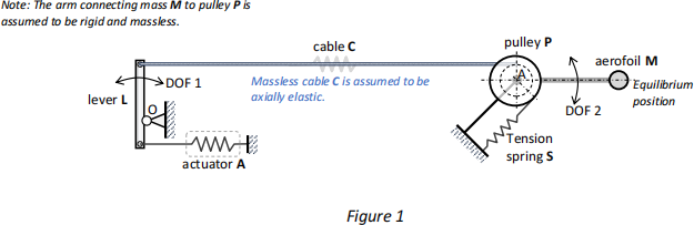
Specification: A wind tunnel installation used to control motion of an aerofoil is described in Figure 1 below. The system consists of an actuator A, lever L, cable C, pulley P, tensioning spring S and aerofoil M.
Assumptions: A is modelled as a linear spring; L is rigid, has nonzero mass and pivots about point O; C is axially elastic and massless, P has nonzero mass and rotates about point A; M is modelled as a point mass rigidly connected to P using a massless arm; S is a linear spring. The system is in equilibrium as shown, friction is neglected and any initial pre-tension in the system is ignored. Define your own reasonably chosen parameters as necessary. Assume small angles where necessary.
Solve the following tasks:
• Results section: include your schematic which represents the system and includes all quantities (coordinates and parameters) required to model the system using Lagrange’sapproach.
• Results section: Use Lagrange’s equations to derive the mass and stiffness matrix of the system. Include the full Lagrangian and a brief statement explaining its composition.
• Results section: choose physically meaningful parameter values and a range of the cable C stiffness values, shown them and then plot the variation of the natural frequencies with the cable C stiffness.
• Discussion section: In a short paragraph, qualitatively and quantitatively describe the mode shapes of the system for your chosen value of the cable C stiffness.
• Discussion section: In a short paragraph, describe the trends observed in the natural frequency versus cable C stiffness plot. What is a possible practical use of these insights in dynamic design?
Guidance, suggestions, hints:
• Recommended layout: Results section 3/4 A4 page, Discussion 1/4 A4 page
• Apply the Newton’s method, assume small angles/linearise, obtain matrices, perform eigenvalue analysis using eig function in Matlab (or solve the characteristic equation).
• Each discussion point typically ranges between one and two sentences which should cover a useful or interesting insight into the specified aspect of discussion.
• Main recommended resources: lectures 11, 12; lectorial recordings; “Matlab and vibrations - … revision note”, example sheets.
Task 5: Transient aeroelastic simulation of 2 DOF system (20% of 100%)
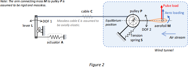
Specification: Consider the system from Task 4 and perform further aeroelastic analysis. Here, as shown in Figure 2 below, assume that the aerofoil M generates a quasi-steady aerodynamic loading concentrated in the centre of mass. As described in the bullet point list below, perform the transient aeroelastic analysis due to a chosen pulse loading. Assume small angles where necessary. Define your own reasonably chosen additional parameters as necessary.
Solve the following tasks:
• Results section: show the sketch used to develop the analytical expressions. Also show the resulting quasi-steady aerodynamic and pulse loading. Finally, show the derived generalised loads.
• Results section: show the overall aeroelastic damping and stiffness matrices.
• Results section (include Appendix for this section to be marked): Choose your own remaining parameter values, show them, and then implement the model in a programming environment of your choice (e.g., Matlab). Solve the aeroelastic system numerically under the influence of impulse loading and show the transient response for two different values of an arbitrarily chosen problem parameter of practical significance.
• Discussion section: In a short paragraph, explain the reason for choosing the above parameter of practical significance and outline the resulting main trends.
• Discussion section: In a short paragraph, describe the possible implications and required model improvements when assuming large angles in terms of further refined aeroelastic analysis.
• Appendix (one additional page expected): include a copy of the working Matlab code which you developed and used to solve the transient aeroelastic response.
Guidance, suggestions, hints:
• Recommended layout: Results section 3/4 A4 page, Discussion 1/4 A4 page
• Use quasi-steady aerodynamic theory to determine the aerodynamic loading.
• Possible impulse load shapes: Heaviside-based pulse, 1-cosine, parabolic, triangular, etc.
• If using Matlab for this task, ode45 can be used to calculate the dynamic response of the system.
• Use the state equation of ideal gas and isothermal conditions to calculate the pressures.
• Main recommended resources: lectures 10, 16, 19, 22; lectorial recordings; “Matlab and vibrations - … revision note”, M-files in “Matlab” folder.
Appendix
Background and context
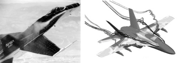
“Fighter aircraft have been designed to fly and maneuver at high angles of attack and at high loading conditions. At these high angles of attack, the flow separates from the sharp leading edges of the wing and leading-edge extension (LEX) forming a strong vortical flow that maintains the stability of the aircraft. However, the leading-edge vortices breakdown upstream of the vertical tails. The breakdown flow impinges upon the vertical tail surfaces causing severe structural fatigue and has lead to their premature fatigue failure, costing millions of dollars every year for inspections and repairs.” [Sheta&Huttsell, 2003]
Moses, RW, Active vertical tail buffeting alleviation on a twin-tail fighter configuration in a wind tunnel, CEAS International Forum on Aeroelasticity and Structural Dynamics. 1997.
Sheta, EF, Huttsell, LJ., Characteristics of F/A-18 vertical tail buffeting. Journal of fluids and structures, 2003 Mar 1;17(3):461-77.
Within the context of this coursework, you area vibration specialist asked to analyse a problem of all-moving vertical stabiliser buffeting on a sixth-generation fighter aircraft. A range of tasks needs to be completed to characterise the system and propose the viable passive vibration control solution based on the application of the tuned vibration absorber concept.
The technical tasks have the following focus (detailed description in the main body of this document):
1. Single DOF analysis using the provided Matlab model.
2. Two DOF analysis using the provided Matlab model and eigenvalue analysis.
3. Vibration absorber tuning combined with the use of the provided Matlab model.
4. Derivation of the equations of motion for a new two DOF system.
5. Transient aeroelastic response using own Matlab simulation with the impulse forcing.
To complete the first three tasks, the provided Matlab application model (called “app”) will be used as a form of a “digital twin” which represents the overall system with the unknown vertical stabiliser properties (later also called “ wing” or “aerofoil”). The last two tasks are independent of the provided Matlab app.
The tool and the modelled system
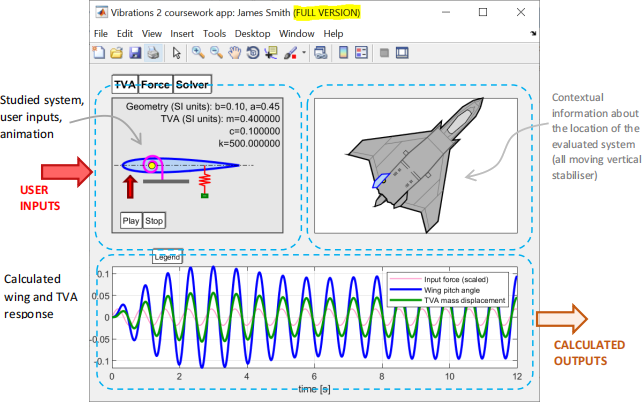
To support the first three tasks of this coursework, a simple Matlab app is provided in the P-file format to avoid the necessity or possibility of the source code modification. The app represents a model of the problematic vertical stabiliser with the unknown physical properties which will be determined in Task 1.
The system’s visual representation is shown in the following figure together with its constituent components, model elements and relevant geometry information (note the offset dimensions).

This is a two degree-of-freedom problem where the first DOF is realised by the aerofoil pitching and the second DOF is linked with the vertical motion of the TVA mass.
The application window is shown in the following figure where the main user blocks are identified and described.
IMPORTANT: You must use the FULL version of the Matlab app which can be downloaded from “Assessment
Information” folder located in “Assessment, submission and feedback” section. In the FULL version, all students have their own individual aerofoil parameters to work with.
User functionality
After each user-specified parameter update, the system’s vibration response is automatically updated and shown in the bottom panel. The user inputs are applied in the top left panel. The top right panel serves for simple contextual information about the overall system layout.
The user input windows can be activated by a mouse click on: “TVA” or the spring-mass visualisation of the damped TVA (see figure below) to change the mass, damping and stiffness of the TVA; “ Force” or the red arrow visualisation of the input force to change the time-dependent excitation function (see the figure below); “Solver” to adjust the ODE time integration range, discretisation and the initial conditions.

The time-dependent excitation function can be any valid Matlab expression with the specific parameter values and a time symbol “t”. Examples of suitable functions are: “ 1” (a constant unit step at t=0 sec), “30*sin(2*pi*3*t)” (a harmonic force at 3 Hz), “0” (a zero-force leading to free vibrations for the non-zero initial conditions), “0.1*t” (a slow ramp function). More complicated function specifications are possible. The four initial conditions represent: (1) initial aerofoil angular displacement in [rad]; (2) vertical TVA displacement in [m]; (3) aerofoil angular velocity in [rad/s]; (4) vertical TVA velocity in [m/s].
For precise analysis purposes, the calculated vibration responses can be plotted separately after a mouse click on any of these lines. A separate window will be generated which will show the applied force in [N] (the top subplot). The bottom subplot contains the aerofoil angular displacement (shown in blue) in [rad], and the vertical TVA mass coordinate (shown in green) in [m].

A mouse click on one of the calculated vibration response curves also updates the content of the variable “var_tvalab” which is present in the base workspace (i.e., through command line) and can be used for further analysis in or outside of Matlab. The columns in this matrix represent [time,dof1,dof2,force] and the rows represent the time instants for which the responses were calculated.
An animation of the obtained responses can be started (stopped) by clicking on “Play” (“Stop”) text fields. A click on “Legend” text field switches on/off a legend in the calculated vibration response panel.
App start and initial configuration
Each student must download their own FULL version from the “Assessment Information” folder located in the “Assessment, submission and feedback” section of the unit to be able to work with their own problem specification. In other words, every student has their own specific aerofoil parameter values to determine in Task 1.
The FULL version of Matlab app must be started using a single input argument which represents the student’s “UOB USER NAME” typed in lower case on the Matlab command line. The P-file must be located in the directory visible to Matlab, e.g., current working directory.
Example:
vib2_tvalab_2023c_full('js00000') % use your own UOB USER NAME
After this, the application starts and is ready to be used for further analysis:

The default initial state of the app is represented by the student’s specific aerofoil parameters, the identical and adjustable TVA parameters, and semi-randomised harmonic excitation force. The force and TVA parameters can be changed. The aerofoil parameters are fixed and specific to each student.
Final remarks: It is recommended to run the app on your own machines, assuming you have a Matlab installation. However, in case of problems of any kind on your local machines, you can work with this app on your own UOB remote desktops. This option was assessed and was found to be a feasible option for the use of this tool. This Matlab app does not assume or require the use of any special toolbox, only the core Matlab functionality is used.
2023-12-25