Computational Finance Fall 2023 Homework 2
Hello, dear friend, you can consult us at any time if you have any questions, add WeChat: daixieit
Computational Finance Fall 2023 Homework 2
Question 1
In this problem, we will further develop our understanding of mean-variance portfolio op- timization that you started in your Investments class and continued in this week’s lecture. Specifically, we will assess how the correlation between two assets affects the tangency portfo- lio. Our goal will be to plot tangency portfolio weights as a function of the correlation.
In the last section of efficient_frontier.ipynb notebook (which closely follows what we did in class), you will see an interactive widget – like the one we saw in the retirement.ipynb example in the first class. This widget allows you to change the correlation between two assets and see how the efficient frontier, tangency portfolio, and the CML change. Every time you change the correlation rho, you are calling the calc_optimal_portfolio() function that recomputes and replots everything.
Even though it is nicely interactive, it is not a particularly efficient. Let’s vectorize the code so that we can compute the tangency portfolio weights for a range of correlations all at once.
Part A: Define Variables
1. Store expected returns and volatilities of the Intel and National Instruments into vectors.
2. Define an evenly spaced vector of weights for Intel between 0 and 1 in increments of 0.0001.
3. Define an evenly spaced vector of 500 correlations between -0.95 and 0.95.
Part B: Calculate Tangency Portfolio Weights
1. Calculate returns and volatilities of the portfolio for each pair of weights and correlations. This will effectively calculate 500 efficient frontiers, one for each correlation. Use vectors and matrices, and take advantage of broadcasting. Do not use for loops.
Hint: Store weights in a (1,N) 2D ndarray and store correlations in a (M,1) 2D ndarray. Then, use broadcasting to create a (M,N) 2D ndarray of, for example, portfolio volatilities.
2. Calculate the slopes for every CAL for every correlation.
3. Approximate the slope of the efficient frontier at every point for every correlation.
4. Find the tangency portfolio weights for every correlation. Hint: In class we used the argmin() method to do this. Here, you can use this same method and specify the axis argument.
Part C: Plot the Tangency Portfolio Weights
1. Plot the correlation on the x-axis and the tangency portfolio weights on the y-axis. You should have two lines, one for Intel and one for National Instruments. Don’t forget to label everything appropriately. Check your results against the interactive widget in efficient_frontier.ipynb. If your results don’t match, see if you can fix your mistake.
2. Describe the relationship you see in the plot. What happens to the tangency portfolio weights as the correlation increases? Why?
3. Notice that by considering only weights between 0 and 1, we are implicitly assuming that short-selling is not allowed. If we could sell short, would the efficient portfolio weights change? For which correlations would they change? How can you modify your code to allow for short-selling?
Question 2
In Week 1, we used Python to analyze the main personal finance problem facing most individ- uals – saving for retirement. In this question, we will tackle the other – buying a house.
Suppose you want to get a 30-year mortgage on a $400,000 home. You can get a 7.1% annual mortgage rate that is compounded monthly when you make a 20% down payment (so the initial loan principal will be $400,000 minus 20% of that value).
The fixed monthly payment PMT on a mortgage is given by the annuity formula:
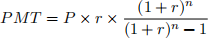
where P is the initial principal, r is the monthly interest rate, and n is the number of months in the mortgage term.
Each payment consists of a principal and an interest component. The interest is akin to a coupon payment on a bond, compensating the lender for risks and time value of money. The principal payment gradually reduces the outstanding balance of the loan. The gradual repayment of principal is known as amortization. It occurs for mortgages but not for bonds, where the entire principal payment, or face value, is paid at the end of the loan as a balloon payment.
The interest component of the payment is calculated as the outstanding balance of the loan at the start of the month times the monthly interest rate. The principal component is the difference between the total payment and the interest component. In other words,
INTt = Bt−1 × r
PRNt = PMTt − INTt
Bt = Bt−1 − PRNt
where INT is the interest portion, PRN is the principal portion, and Bt is the outstanding balance of the loan at the end of month t. B0, the initial balance, is the initial loan amount P.
Part A: Calculate the Amortization Schedule
1. Calculate and print out the following values:
• The monthly payment (note: the payment shold be rounded to dollars and cents not just for printing but for calculating as well. The bank won’t charge you fractional cents.)
• The final payment (it may not be exactly the same as the payment in all other months because of the rounding you did above)
• The final balance (it should be zero – if not, find and fix your mistake)
• The total interest paid over the life of the loan
• The total principal paid over the life of the loan
• The total payments over the life of the loan (sum of interest and principal)
2. Display a plot of the principal balance over time with the year on the x-axis and the balance on the y-axis. Label appropriately, here and elsewhere.
3. In a different plot (but could be part of the same figure if you optionally use subplots(1,2)), plot both the monthly principal payment and the monthly interest payment with the year on the x-axis. Label the plot appropriately and include a legend. Eyeballing the plot, at approximately what year do the principal and interest payments cross?
Part B: Choosing Points
You have the option to buy “points” on the loan. This means that you can pay an extra 1% of the initial principal along with your down payment, and doing so will lower the annual interest rate by 0.25% (thereby lowering the monthly payment). Importantly, the points you pay – the extra 1% – do NOT count towards the principal of the loan. They are just a fee paid to the bank. In exchange, you get a lower interest rate. Lenders will often advertise the lower rate, to get whcih you need to pay the points. But is it worth it? You will figure this out in this question.
If you own the home for the entire 30-year loan period, buying points usually lowers the total cost of the loan. But most people don’t do that – they often move before then. When you sell the house, you use (some of) the proceeds from the sale to repay the remaining mortgage balance, after which you no longer need make any payments.
Suppose you decide to sell the house after living in it for k months (and making k monthly payments). The total cost of the mortgage is the cost of points paid today, plus k months of monthly payments PMT , plus the final balance at the end of the kth month Bk .
The total cost of the mortgage is then:
TC = points × P + PMT × k + Bk
Of course, as an experienced finance student, you know about time value of money, which means that you shouldn’t make decisions based on discounted total costs of many payments over time. So given a monthly discount rate rinv, you compute the present value of mortgage payments as:
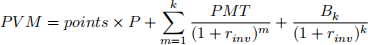
What discount rate should you use? This is the age-old question in finance. One way to approach it is to discount cash flows at your opportunity cost, i.e. at the rate you can earn on an alternative investment of similar risk. Intuitively, the reason why money 10 years from now is worth less to you than money today is because, if you got money today, you could invest it and have more in 10 years. Let’s assume an annual discount rate of 4%.
1. In a new part of your notebook, rearrange (“refactor”) your code from Part A into a function that takes points, interest rate, and the months until you sell the house as inputs and returns the present value of the mortgage as an output.
2. Assuming 1 point (1%) buys you a 0.25% reduction in the annual interest rate, use your function to igure out when it is worth to pay points and when it is not, depending on how long you plan to live in the house (k). Print and/or plot whatever results you find helpful in getting to your result. For example, you may find it useful to plot the present value of the mortgage as a function of k, for both the case with and without points.
2023-12-21