Coursework 3 – Goodness of fit and Monte Carlo Sampling
Hello, dear friend, you can consult us at any time if you have any questions, add WeChat: daixieit
Coursework 3 – Goodness of fit and Monte Carlo Sampling
Part 1: Goodness of fit
The univariate sample data to be used for questions 1 to 5 is in the file cw3_data.txt on Black-board which contains only one column.
There are n = 120 observations in the dataset. You should firstly read the data into R from the named txt file.
We want to investigate whether the data could be regarded as a random sample from a Normal distribution. To this end, you should standardise the data using the sample mean and standard deviation. We will then look at whether the standardised data can be regarded as a random sample from a N(0, 1) distribution.
1. Produce a histogram of the standardised data and superimpose a kernel density estimate and a N(0, 1) pdf. Comment on the goodness-of-fit. [3]
2. Manually construct (rather than using an existing R function for this purpose) a Normal quantile-quantile plot of the standardised data and superimpose a suitable reference line to help gauge Normality. Comment on the form of your plot and relate it to your results in Q1. Say whether you think that Normality was a tenable assumption or not. [4]
3. We now wish to carry out a Kolmogorov-Smirnov (KS) test to assess whether the distribution of the standardised data is N(0, 1). Find the value of the KS test statistic for this test and also that standardised data value where the absolute di↵erence between the empirical and N(0, 1) cdfs is a maximum. Report these values. [3]
4. Produce a plot containing the empirical cdf of the standardised data and the N(0, 1) cdf and indicate on it the point at which the maximum di↵erence between the two distribution functions occurs. [3]
5. (i) Write a function in R to simulate the sampling distribution of the Kolmogorov-Smirnov test statistic when the N(0, 1) null distribution is true using the same sample size as that of the sample data. [3]
(ii) Run your function and use the results to plot a histogram of the estimated sampling distribution with a superimposed kernel density estimate of this distribution. Comment on the plot. [2]
(iii) Use your simulated test statistic values to obtain an estimated 5% critical value for your test. Indicate this value on your plot from Q5(ii). Compare your observed value with this critical value and report your conclusions. [2]
Part 2: Monte Carlo Sampling
6. Express the integral
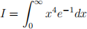
as E(h(x)), where h(x) is to be determined and use Monte Carlo integration to approximate I. Report the Monte Carlo estimate and its estimated standard error. Based on your resulting estimate,  , propose a Monte Carlo estimate for the Gamma function Γ(5) and comment on the results. [5]
7. Consider the mixture Normal distribution with pdf
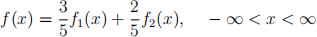
where 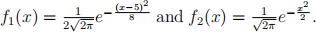 We would like to use rejection sampling to obtain a sample of size N from the mixture Normal distribution and based on that sample, estimate the probability P(0 <x< 5) via Monte Carlo Integration.
(i) Assume a Normal proposal N(2.5,10) with pdf 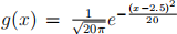 for your rejec-tion sampling scheme, and determine a suitable value for the bound M, by visually comparing f(x) with Mg(x) for M = 1, 1.5, 2, 2.5, 3. [2]
(ii) Write a function in R to simulate a sample from f(x) using the proposal g(x) and M.
Your function should output
– Your simulated data
– The acceptance probability of the rejection sampling algorithm
– A plot comparing the density of the simulated data to f(x) [4]
(iii) Run your function to obtain a sample of size N from the mixture Normal distribution. Report your acceptance rate and comment on the plot. [2]
(iv) Use the sample to obtain a Monte Carlo estimate of P(0 <x< 5). Report your estimate along with a 95% Confidence Interval.
Hint: Express P(0 <x< 5) as E(h(x)), where h(x) is to be determined. [2]
2023-12-19