Hello, dear friend, you can consult us at any time if you have any questions, add WeChat: daixieit

2/ Theory

2-1/ Apparatus

The apparatus consists of two discs welded together, mounted on a horizontal shaft and connected to a tachometer. The full apparatus being mounted on the laboratory bench. The tachometer measures the angular speed of the shaft o (in rad/s). The output of this tachometer is fed onto a data acquisition system which displayso(t) curves. In the

first experiment, the falling mass, shown in figure 1, is not attached to the discs and the free-wheeling rotation of the discs is observed. In the second experiment, the mass is attached and, once again the o (t) curve is recorded.

Note that in this second experiment you will also need to measure the initial height h of mass m with respect to the laboratory floor and count the number of revolutions the discs keep turning once the mass has hit the floor.

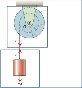
Figure 1: Two sub-systems present in the apparatus, the welded discs and the falling mass.

2-2/ Moment equation for a rotating rigid body

At equilibrium (no angular acceleration), the sum of the moment of the external forces on a rigid body is zero. In the general case (ie no equilibrium), the sum of the moment of the external forces is non-zero and is equal to the product of the moment of inertia and the angular acceleration. This equation is the rotational equivalent to Newton’s second law, as shown in figure 2. The moments of the forces M plays the role of the forces F (cause of motion), the moment of inertia I plays the role of the mass m (resists motion) and the angular acceleration a plays the role of the linear acceleration a (describes the resulting motion).

Figure 2: comparison between Kinetics translation and rotation equations

A solid cylindrical disc of mass M, and radius R has a mass moment of inertia I=(M/2). R2. In the laboratory, we only consider the I value of the object shown in figure 3. The moment of inertia of this system is the sum of the moments of inertia; i.e. moment of inertia of disc 1 + moment of inertia of disc 2. Finally, note that, in general a moment of inertia is defined with respect to an axis, in the present case the axis going through the pivot O, perpendicular to the discs, and we should really call it Io, but for brevity we will simply adopt the letter I.

Figure 3: rotating system in the laboratory is made of two discs welded together.

2-3/ Calculation of theoretical angular acceleration

The apparatus can be described as two mechanical sub-systems, the welded discs and the falling mass, as shown in figure 1. While the welded discs will obey the moment equation, the falling mass will obey Newton’s second law. In addition, there will be a kinematic relationship between the motion of the disc and that of the mass. Assuming to slippage and/or extension of the rope, a=R.a, where R is the radius of the inner disc (R2).

3/Experimental procedure to use the DMS2 data acquisition board

To use the DMS2 data acquisition board, the two leads of the tachometershouydl be connected to the AC1 input on the DMS2 data acquisition board. The serial port on this board should be connected to the back of the computer’serial port , see figure 4.

 

Figure 4: connections from the tachometer to the DMS2 (left) an from that board to the computer (right).

Open the data acquisition software (DMS2 icon on the desktop). Figure 5 shows the main controls on top of the screen.

Figure 5: Main controls on opening the DMS2 software.

Press File/layout/Open custom layout/ angular velocity measurement, as shown in figure 6.

 

Figure 6: To open the customized ‘angular velocity measurement’ layout.

Press Connection and ‘connect to device’ .

Before starting an acquisition on the DMS2 software, DO THE FOLLOWING

DATA/VIEW DATA TABLE/DELETE CURRENT DATA SERIES  this is to empty the data buffer so that only one acquisition is saved.

To initiate an acquisition, press the ‘clock/green arrow’ icon, this brings a window as shown in figure 7

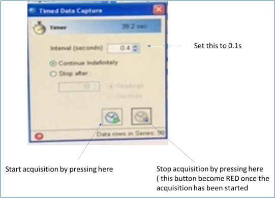
Figure 7: Window appearing on starting an acquisition, permitting to set the acquisition parameters.

Set the time interval to 0.1s, press ‘Continue Indefinitely’ . MAKE THE WHEEL TURN, by pulling on the rope

(experiment 1) or letting the mass fall (experiment 2). You can stop the acquisition by pressing the red button.

For both experiments, this will after the wheel has stopped turning.

Once the acquisition is completed;

Press file/Export to HTML

When the ‘SAVE AS’ window appears, press SAVE

When the ‘ File already exist, append new data?’ window appears, press NO

This will generate an HTML file with two columns; t (s) and angular speed (rad/s).

Press  CTRL  A  (select  all),  then  CTRL  C  (copy).  Then  you  can  paste  this  onto  an  empty  Microsoft  Excel spreadsheet, removing the first three rows, as shown in figure 8 and rename the new first row as t,s and omega, rad/s..

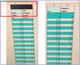
Figure 8: After exporting data onto spreadsheet, remove first three rows (left) to get the data in the format shown on right.

4/Instructions for carrying out the measurements

Experiment 1- free-wheeling acceleration

Make sure no mass is attached to the pulley. Make an acquisition using the procedure explained in 3/, main steps are reported below;

1.    Wrap the string around the disc, ensuring that it is free to pull off the pulley.

2.    Start the data acquisition by pressing the green button on this panel

3.    Accelerate the disc up to a reasonable speed by pulling on the string.

4.   Allow the disc to decelerate naturally to a standstill

5.    Once the disc has stopped rotating, you can stop the data recording by hitting the red button.

Use section 3/ to export the data, repeat this acquisition three times.

Experiment 2- falling mass acceleration

Figure 9 shows the starting position of the mass, before the fall, to ensure that the metal hook is not rubbing against the bench.

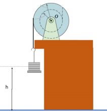
Figure 9: Experiment with the falling mass showing the initial position with the hook just below the bench.

The height h represents the distance from the mass center of the weight to the laboratory floor.

1.    Again, take the piece of string and wrap it around the disc (on the smaller diameter), ensuring that it is free to pull off the pulley.

2.    Hang a known weight of around 500g from the end of the string in the position shown in figure 6 (h~ 78.5 cm) but prevent it from falling by holding the disc.

3.    Start the data acquisition by pressing the green button on this panel

4.    MAKE SURE EVERYONE STANDS BACK FROM THE MASS AND THAT NO ONE IS AT RISK OF BEING HURT BY THE

FALLING MASS.

5.    Release the mass, allowing it to fallonto the ground

6.   The string should unwind fully from the disc, and fall away. Now allow the disc to decelerate naturally to a standstill

7.    Once the disc has stopped rotating, you can stop the data recording by hitting the red button.

Use section 3/ to export the data. repeat this acquisition three times.

5/ Use of Microsoft Excel to derivate and integrate quantities

The only data you export onto the spreadsheets are o(t) curves. Firstly, you will sometimes be asked to calculate the angular

acceleration, which represents the slope of that curve and corresponds to a derivation operation. Secondly, you will be asked to calculate an angular displacement which represents the area under the curve and corresponds to an integration operation.

Acceleration/slope/derivation:

You will have to select the ‘time interval of interest’, as the recorded data often includes much more data. For instance, if you are calculating the angular deceleration for the free-wheeling discs, you must remove the data points at the start corresponding to the acceleration of the discs when your hand is still on the discs and also remove the data after the disc has stopped. If you are analyzing the angular acceleration due to the falling mass, you must remove the data points at the start corresponding to   instants just before you dropped the mass and instants after the angular acceleration has reached its maximum. Examples are shown in figure 2 and 3.

 

Figure 2: for calculation of the free-wheeling deceleration value from the slope, delete all data outside the region of interest; remove data in RED..region of interest shown on the right

 

Figure 3: for calculation of the acceleration due to the falling mass from the slope, delete all data outside the region of interest; i.e. remove data in RED.. region of interest shown on the right

To calculate the slope, click on the data points and ‘add trendline’ choose a ‘linear fit’, select ‘display equation on chart’ and ‘display R2 value on chart’ .

To calculate a standard deviation on the slope value, use the LINEST function in excel, which you can find on the following link

https://www.youtube.com/watch?v=Y-rfyeutais

Angle/area/integration:

You will have to select the ‘time interval of interest’, as the recorded data often includes much more data. For instance, if you are calculating the angle after the mass has hit the floor, you must remove the data points at the start corresponding to the acceleration of the discs while the mass is falling and also remove the data after the disc has stopped. An example is shown in figure 4.

 

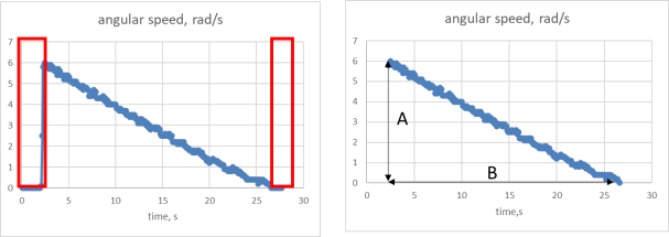
Figure 4: for calculation of the angle during free-wheeling, after the mass has hit the floor, delete all data outside the region of interest; i.e. remove data in RED..

Once this is done, you want to integrate the area under the curve. You have two options

Option1: IF YOU CAN ACCESS THE FUNCTION QUADXY (Calculus ADD-IN), use the link below:

https://www.youtube.com/watch?v=QDhD01IPDz4

The procedure is as follows. Let’s assume your time data is from cell B2 to cell B50 and that the angular speed data is from C2 to C50. Then, use any empty cell on the spreadsheet and type

=QUADXY (B2:B50,C2:C50) and press ENTER

The number you get is the value of that integral, the full angle. If indeed the time was in second and the angular speed in rad/s, it will bean angle value in radian. To get the number of turns, divide by 2π, divide by 6.283.

Option2:

Retain only the data of the region of interest to calculate the angle. It should be approximately a triangle.

Hence the area is A x B/2, referring to figure 4, where A is a speed in rad/s and B a time in second, the area being in radian.