This problem set uses simulation experiments to study the performance of OLS and IV estimators. In each of the settings that you will consider, the parameter of interest is β, the causal effect of one “treatment” of interest on a hypothetical outcome Y.

For each data generating process (DGP) that you consider, write a Stata program that repeatedly (say, 10,000 times) creates a dataset drawn from the DGP and records the value of any estimators computed with each dataset replication [note, while debugging your code, keep the number of repli- cations set to a low number, and only increase it to 10,000 for final runs].  Then use this program to complete the following simulation experiments investigating the finite-sample properties of the vari- ous estimators. This will usually involve repeating the simulation exercise under a number of different parameterizations of the DGP. [Note, the example code I provide is in Stata, but you can use another language if you prefer.]

Your solutions should be typeset and include a written discussion/explanation of your results in addition to any supporting tables and figures. Please also submit the final code that you use to produce these results.

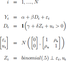
A. Continuous instruments and a continuous endogenous regressor:

Consider the following data generating process.

1.  Under what values for the model’s parameters will estimating the first equation directly by OLS yield a consistent estimate of β? Under what values for the model’s parameters would an alternative IV estimator yield a consistent estimate of β?

2.  Use simulations to examine the the performance of the OLS estimator OLS .   Estimate the mean and variance of its sampling distribution. How do these moments compare with those of the theoretical (asymptotic) sampling distribution? How does the mean of βbOLS,k (k indexes replications) depend on ρu? How does the variance of βOLS,k  depend on the sample size N?

3.  First pretend that you only have access to the potential instrument Z2  (the variable Z1  is not available). Use simulations to examine the performance of the IV estimator βbIV based on that single instrument.  Estimate the mean and variance of its sampling distribution for a range of values of ρz2 , including the case where the instrument is valid (ρz2    = 0).  What do you find? How do these moments compare with those of the theoretical sampling distribution?

4.  Continue under the assumption that you only have access to the one potential instrument Z2 . Using simulations, illustrate how the mean and variance of IV,k  depend on δ2 .  Be sure to include some cases where the instrument is weak (δ2  is small).

5.  Now, making use of the instrument Z1 that you know is a valid instrument, simulate a Hausman test of the null hypothesis that Z2  and Z1  are both valid instruments against the alternative that only Z1  is a valid instrument. Record the fraction of tests that reject the null hypothis (fallin the asymptotic rejection region) at the 5% confidence level.  What is the rejection rate when ρz2   = 0, and what is the rejection rate as ρz2       0 increases in magnitude.  If you didn’t know the statistical properties of Z1  and Z2 , would the Hausman test be helpful in learning whether you had two valid instruments?

B. Binary instrument and a binary endogenous regressor:

Consider the following data generating process.

1.  Propose a Wald estimator for β, called IV 1, that makes use of the available instrument Z. Sim- ulate the performance of this estimator, and compare it to the two stage least squares estimator that you can compute directly using “ivreg.” Do you prefer one of the estimators to the other?

C. Two binary instruments and a binary endogenous regressor:

Consider the following data generating process, which is similar to the one from part B., but with two added wrinkles.  Now the treament effect β is not the same for all individuals i, and you have access to two potential instruments.

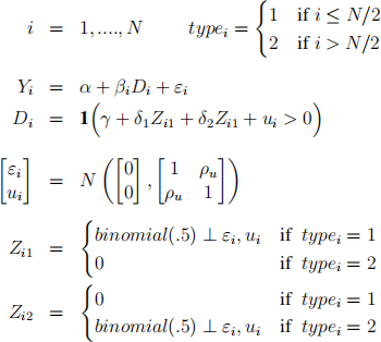
1.  Using this setup, simulate data where the “treatment effect” β differs between the two types of individuals.  Specifically, set the parameter βi   = 1 for those with typei   = 1 and o set the parameter βi  = 2 for those with typei   = 2.  Simulate the sampling distribution of βIV  using only Z1 as an instrument, the sampling distribution of IV  using only Z2  as an instrument, and the sampling distribution of IV  using both instruments simultaneously.  Do you get similar results using the different IV approaches?  Explain what is going on.  Which of the three IV approaches do you think is correct?

2.  Simulate a Hausman test of the null hypothesis that Z2 and Z1 are both valid instruments against the alternative that only Z1  is a valid instrument. Record the fraction of tests that reject the null hypothis (fall in the asymptotic rejection region) at the 5% confidence level.  What do you make of this result. In the data that you simulated, are Z1  and Z2  in fact valid instruments?  If you didn’t know the statistical properties of Z1  and Z2 , would the Hausman test be helpful in learning whether you had two valid instruments?