Hello, dear friend, you can consult us at any time if you have any questions, add WeChat: daixieit

Final Examination

Math 422

Fall Semester, 2023.

1.  Suppose that y  = y(x) satisies a second-order homogeneous ODE that has a regular singular point

at x = 0, with characteristic exponents s , s, and a regular singular point at x = 1, with exponents

s , s. There will be four Frobenius series: two coming from the point x = 0, and its two exponents; and

two from the point x = 1, and its two exponents.

Consider the modiied function ˜(y)(x) = xδ y(x). It too will satisfy a second order homogeneous ODE, with

regular singular points atx = 0 and x = 1.

(i) What will the two exponents of this new ODE atx = 0 be?

(ii) What will the two exponents of this new ODE atx = 1 be?

Hint: Part (i) is not hard at all: consider the effects of multiplying each of the two Frobenius series coming from x = 0 by xδ. Part (ii) may require signiicantly more thought.

2. The associated Legendre ODE appears as equation (173) of §4.12. It is a generalization of the Legendre ODE, and has two parameters.  These are the usual n = 0, 1, 2, . . . , and a new integer parameter m, which in most applications is allowed to take on only the values −n,−n + 1,... , n − 1,n.  When m = 0, the associated Legendre ODE reduces to the usual Legendre ODE.

Like the Legendre ODE, the associated Legendre ODE has three regular singular points:  x = ±1 and the point x = ∞ . Compute the characteristic exponents of each of these points.

Hint: By symmetry, the exponents of the singular point x = −1 are the same as those of x = 1; so you need only to compute the exponents of x = 1 and x = ∞ .

3. Consider the function fǫ(x) that equals 1/ǫ on the interval (−ǫ,ǫ), and is zero elsewhere. Here, ǫ signiies a small positive number.

(i) Obtain a complete Fourier series of period 2ℓ, representing fǫ(x) on the interval (−ℓ,ℓ). That is, compute the coeficients A0, A1 , A2 , . . . and B1, B2 , . . . , in the notation of §5.11. You should assume that ǫ < ℓ .

(ii) Similarly, obtain a complete Fourier series of period 2ℓ, representing δ(x) in the interval (−ℓ,ℓ).

(iii) As ǫ → 0, the function fǫshould converge (in a ‘weak’ sense) to the singularity function Cδ, where C is a certain constant. Determine what C is, by examining the coeficients computed in (i) and those computed in (ii). The former should converge to C times the latter, when ǫ → 0.

Hint: In part (iii), L’Hˆopital’s rule maybe useful.

4. Many special functions have integral representations: formulas that express them as deinite rather than indeinite integrals.  (The argument of the special function appears as a parameter in the integrand.)  One such representation for the order-zero Bessel function J0(x) is

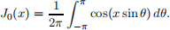
That is, J0(x) is the average value of cos(xsinθ), which by examination is an even function of θ with period 2π, on the interval −π < θ < π. Or to put it differently, if one expanded cos(xsinθ) in a complete Fourier series of period 2π, representing cos(xsin θ) on the interval (−π,π), the coeficient A0  (which depends on the parameter x) would be J0(x).

Show that this is plausible, in the sense that if y = y(x) is the right-hand side, theny will satisfy the p = 0 case of the Bessel ODE

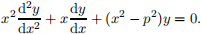
Hint: An integration by parts maybe useful.

Comment: Because any Bessel ODE has a two-dimensional space of solutions, to provide a full proof that the representation formula is valid, one would need to check that the right-hand side of the formula deines the solution that we call J0(x), and not some other solution. But it turns out that it is.

Comment: It also turns out that the Bessel functions of higher order, Jn(x), n ≥ 1, are related to the higher Fourier coeficients An , n ≥ 1.

5. The seldom-used ‘parabolic’ coordinate system on R3 uses coordinates (ξ,η,ϕ) which in a sense liebe- tween spherical and cylindrical coordinates. Theirst two coordinates ξ,η equal r−z andr+zrespectively, where r = ^x2 + y2 + z2 , and the third coordinate ϕ is the usual azimuthal angle: the longitude, i.e., the angle around the z-axis.

By changing variables from (x,y, z) to (ξ,η,ϕ), it can be shown that the Laplacian operator ▽2 on R3 can be written in terms of parabolic coordinates thus:

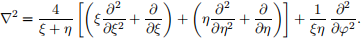
The Helmholtz equation ▽2 f − f = 0 is a PDE that is a modiied version of Laplace’sequation. (It is often written as ▽2 f + k2 f = 0 where k2 is a free parameter, but for simplicity, k2  is taken to equal −1 here.) Like Laplace’s equation ▽2 f = 0, the Helmholtz equation separates in many coordinate systems, and one of them is the just-described system of parabolic coordinates.

(i) To prove this, consider a ‘product form’ solution f = fp(ξ,η,ϕ) = 工(ξ)H(η)ϕ(ϕ) of the Helmholtz equation, and in particular (to keep things simple), consider an axisymmetric solution that does not depend on the azimuthal angle ϕ, i.e., f = fp(ξ,η,ϕ) = 工(ξ)H(η). Substitute f = fp into the Helmholtz equation, and multiply the entire resulting equation, term by term, by (ξ + η)/fp.  The terms on the left-hand side should then be of two types: ones that depend only on ξ, and ones that depend only on η. The sum of the ξ terms must therefore equal a constant (the ‘separation constant’), and the sum of the η terms must equal its negative. In this way, derive a second-order ODE satisied by 工(ξ), and a very similar second-order ODE satisied by H(η).

(ii) Substitute 工(ξ)  = L(ξ)exp(−ξ/2) into the just-derived ODE satisied by 工(ξ), and show that the function L(ξ) must satisfy Laguerre’s equation, which is the ODE given in Problem 24 of Chapter 4  [or Problem 17 in the irst edition].  So, Laguerre functions, like many other (but not all) well-known special functions, can arise in the method of separation of variables, applied to well-known PDE’s.