PHY254 Computational assignment Fall 2023
Hello, dear friend, you can consult us at any time if you have any questions, add WeChat: daixieit
Computational Assignment
Due 3 December 2023 at 11:59 p.m.
Preliminary question If you haven’t yet, read the “Homework set policy” document in the “Prac-ticalities” module on Quercus. Did you read and understand the policy? If you did, write down
“I have read and I understand the homework set policy in this course.”
in your copy. You should answer this question truthfully before continuing with this homework set.
In particular, make sure you re-read the policy about code!
For all questions, if we derived a formula during a lecture or in the lecture notes, you may re-use it without justification other than a simple reference to the notes or textbook.
With this assignment, you should be able to download the following Python scripts:
• pendulum_solve_ivp.py,
• find_roots .py, and
• springpendulum .py.
If any or all are missing, let N.G. know ASAP.
Computational questions can be somewhat open-ended, but this does not mean that you should write more than necessary. Aim for concise answers with clearly labelled and described plots. Nu- merical studies are a bit like experiments; you have to try things and report the most interesting things you observe. You do not need to hand in every code you use, otherwise it might be a lot. Instead, hand in a few sample codes that represent your work and will help the marker understand why you find what you find.
We highly recommend saving the code you write for each subquestion below with a different name. For example, when you finish question 2.1, save the code as q21 .py, then save a copy of it as q21 .py and alter this version when you move to part 2 of the assignment. Finally, when you upload code, make sure to reference the script in the body of the text. (E.g., “These figures were computed using MyPrettyCode.py.”)
(DO WE?) We often refer to a certain ddp_routines .py script. It is part of the material for the lecture “Describing chaos”, which we uploaded on Quercus. The functions contained in this script are more advanced that what we are asking you to plothere, but you can reverse-engineer them to suit your needs. You can do a test run on a few of these functions by running ddp_basic_plots .py, making sure ddp_routines.py is in the same directory first.
It is OK to trade code, or to use code we used in class or in the tutorial on the Lorenz attractor, but make sure you understand what you use, and that you manage to express it on your copy. Use your own parameters whenever applicable to show us that you can use the tool. We are training you to use Python for a reason! It is one of the most valuable skills we can teach you, whether it be towards research, industry, or your future coursework.
PHY254
Computational assignment
Fall 2023
1 Comparing methods [20%]
We will now examine the numerical methods that we used to solve problems. Numerical methods occupy an entire branch of mathematics, and depending on the system of equations, these codes can become very large and take years to write.

What happened to !0? Non-dimensionalisation happened, for which a detailed justification and explanation are given in appendix A.
Now we will focus on the numerical methods that we use to solve these problems. Let’s take a step back and use a slightly different method than the one you learned in class. In class, we have been using the Euler-Cromer method of solving F = ma, namely,
If we don’t use the updated value of velocity when calculating position, we are simply using the forward Euler method:
Let’s see what happens when we solve the pendulum using the forward Euler method.
1.1. Write a Python program using the forward Euler method to solve the non-dimensional pen- dulum eq. (1). Use a time step of 0.05τ and plot the energy and θ (on different plots) as a function of time for 60τ. What do you notice? Does this make sense? Why or why not? Now pick a time step of 0.01τ and do the same, what changes? You can pick your initial conditions ![]() (θ(0) and θ(0)) to be whatever you like, but remember that they are in radians and radians/τ . Keep the same initial conditions for each part of this question.
(θ(0) and θ(0)) to be whatever you like, but remember that they are in radians and radians/τ . Keep the same initial conditions for each part of this question.
You should see the energy grow withoutbound for any time step that you can take. While the forward Euler method will produce exact results in the limit Δ t ! 0,for any finite Δ tit is unconditionally unstable for this problem.
1.2. Repeat part 1.1. with the Euler-Cromer method instead of the forward Euler method. What difference do you see between the results from these two numerical methods?
The lesson to be learned here is that numerical methods matter. The forward Euler method won’t fail in all circumstances, it just happens to be particularly ill-suited for problems that have oscillatory solutions. By the same token, the Euler-Cromer method isn’t a particularly good general purpose method either, it just happens to be relatively stable and easy to im- plement.
1.3. With the help of appendix??, examine the program pendulum_solve_ivp.py and make sure you understand it. We know that energy in this system should be conserved, so we can use how much it varies as a proxy for the error in the numerical method. With this in mind, how does the error in the solve_ivp function compare to the forward Euler and Euler-Cromer methods?
Note that the vertical axis in the energy plot may have factored out a multiplication factor for the scale. For the pendulum_solve_ivp.py case there will be a number like +1.999 on top of the y-axis. This means that every number is offset from 0 by 1.999.
2 Rössler system [45%]
The Rössler system is a set of coupled, first order, nonlinear ODEs that can exhibit chaos. It is defined by

where a, b, and c, are constants.
2.1. Write a program in Python to solve the Rössler system by replacing the derivatives on the LHS with finite difference approximations. For example, write

and then rearrange the above x equation for x (t + Δt) = ...). To test that it works correctly, set a = 0.1, b = 0.1, c = 2, x(0) = y(0) = z (0) = 10.0 and Δt = 0.001 and plot x (t) for the first hundred seconds of the system. Your plot should match up perfectly to Figure 1below. If it doesn’t, seek help now!
2.2. Now, compare your forward-Euler method and the solve_ivp method. A tutorial is provided in appendix B, and you may also want to draw inspiration from the solutions of tue tutoria;l on the Lorenz attractor. Try a few different time steps, like Δ t = 0.01, 0.001 and 0.0001. What do you notice?
From now on, you can use whichever method you prefer, as long as you trust it. If you choose the solve_ivp method, we recommend that you use a relative tolerance rtol=1e-7 (cf. Ap- pendix B) for the next questions.
2.3. Now set c = 4 (leave a, b, your initial conditions, and your time step unchanged from the pre- vious question) and plot x (t), y(t), and z (t) for the first two hundred seconds as subplots in

Figure 1: x (t) from the Rössler system for the first 100 seconds of the systems evolution, solved with the forward-Euler method. Here a = 0.1, b = 0.1, c = 2, x(0) = y(0) = z (0) = 10.0 and Δt = 0.001.
the same figure. In dynamics, systems often have to run for a little while before they collapse onto an attractor. When would you say that this system has approximately collapsed onto its attractor? What is characteristic about this attractor (i.e., describe it)?
2.4. Change your program to only plot the solution after the system has equilibrated. Now com- pare the results for c = 4 to the results for c = 6.5 and c = 8 (note: if you change c, the equi- libration time may change). What differences do you notice between these c values? Pay close attention to how long it takes for the signal to truly repeat itself. Considering z maybe helpful in determining this.
The behaviour you observe as c increases is called period doubling, and it is one pathway by which systems evolve into a chaotic regime.
2.5. If we continue to increase c we will find that the time it takes for the system to repeat grows longer and longer and eventually reaches infinity (long before c gets to infinity).
We can visualize this by using the local maxima of z as a proxy for the state of the whole system. Modify your program so that it plots all the local maxima of z as a function of c for a range of c ’s between 4 and 15 (see “Steps to modify your program” below). That is, make a plot of z max vs. c (e.g., if there were 6 distinct local maxima for c = 9 you would have 6 points on the z axis above c = 9 on the c axis). Good results are achieved when you use about 120 values of c between 4 and 15. Run each simulation (one for each c) for about 1300 seconds in order to get enough maxima, and discard the first 250 seconds of each simulation in order to make sure that the solution is on the attractor. This program may take a few minutes to run.
The plot you made is a bifurcation diagram, the regions which are very dense with points correspond to chaotic regions of parameter space. What does this result tell you about the dependence of the system on c?
Steps to modify your program:
• The function getmaxes given below can be used to find the maxima of z. As usual with Python, you should put this function near the beginning of your program.
def getmaxes(z, c):
""" Finds the local maximas in a given solution .
Takes an array z and a float c and returns a list of lists
containing max list and c list .
max list and c list contain the values of all the local maximas in z and the c 's that go with each maxima (the c 's will all be the same for a single getmaxes call) . """
maxlist = []
clist = []
a = (np.diff(np.sign(np.diff(z))) < 0) .nonzero()[0] + 1
for q in range (0 , size(a)):
maxlist .append(z[a[q]])
clist .append(c)
return [maxlist, clist]
• You will want to call the getmaxes function after you have calculated the values of x, y and z. You can call it using:
# Call getmaxes for z
tempmaxes = getmaxes(z, c)
maximas .extend(tempmaxes[0])
cs.extend(tempmaxes[1])
• In order to use this code snippet you will need to define the lists maximas and cs near the beginning of your program with:
# Define the empty lists
maximas = []
cs = []
• Now you will want to create a plot of the maximas vs c. You can do so by adding the following to the end of your program:
# Plot the c 's vs the maximas
plt.plot(cs, maximas, ' o ' , markersize=1.5)
plt.show()
• Finally, you will notice that at this point, the program only works for a single c value. You will want to alter your program so you can loop over a range of c values. To do so, you are going to want to define an outer loop to loop over the c values and put your code that updates the x, y, z stuff and calculates the tempmaxes inside the c loop. Just make sure your plotline is not in the c loop (i.e., is not indented).
2.6. Another property of chaotic systems is a sensitive dependence on initial conditions. Go back to the program you wrote for part 2.3. and rewrite your program so that it solves two Rössler systems simultaneously. You will need two sets of initial conditions, and two sets of time stepping segments. Plot the systems as you did in part 2.3., but plot both x (t)’s on the same subplot, likewise for y(t) and z (t). You can verify things are correct by starting both simula- tions with the same initial conditions, the lines should overlap perfectly.
Add a new subplot which shows the absolute value of the difference between x (t) for the two simulations, if the initial conditions are the same, this difference should be zero.
Note: If you chose the solve_ivp method, you need to force the code to output the solution at fixed times, in order for both arrays of x-values to have the same length and the substraction
to make sense. To do that, create a time array time like we did in class with, for example, the same Δt you used in Q2.2., and add the t_ eval = time option at the end of the solve_ivpcall: solution = solve_ivp( ... , t_eval=time)
were the ... are a placeholder for the other elements of the call we discussed so far.
Now change one of your x (0) by adding 0.0001 to it but otherwise make all the other param- eters the same as in Q2.3. (a = 0.1, b = 0.1, y(0) = z (0) = 10, etc.). Now compare what you see when you set c = 4 and c = 10. What regions of the bifurcation diagram that you found in part 2.5. do these correspond to?
2.7. Write a program to calculate the Lyapunov exponent for the two cases that you looked at in Q2.6. (c = 4 and c = 10) by plotting ln jx1 ¡ x2j for each c, where x1 and x2 are the two slightly different trajectories you plotted in Q2.6..
Remember that in order to calculate the Lyapunov exponent you should only consider the time shortly after your simulation starts. Why is this?
For this question you can eyeball the line of best fitif you like.
3 Springy pendulum [35%]
In this question we will explore the spring pendulum system numerically using Python. This sys- tem consists of a mass on the end of a spring which is free to move in a plane. No small angle approximation is used in this problem so this system cannot, in general, be solved analytically. For certain parameters this system readily displays chaos, exploring this will be the focus of this question.
This is the other kind of chaos that the lecture notes mention: Hamiltonian chaos. There is no forcing, no dissipation, energy is conserved and chaos takes the form of a complete exploration of the accessible phase space rather than collapses onto attractors.
A schematic diagram of this system is shown in figure 2. Here ! is the length the spring stretches to when the weighted system is in equilibrium, !0 is the length the spring is when the unweighted spring is at equilibrium. Finally g and m are the gravity and mass respectively. A coordinate system for this setup can bedefined a number of ways. In this assignment we will use an x-y coordinate system centred at the the equilibrium position of the mass.

Figure 2: A schematic diagram of the spring pendulum system with the mass in the equilibrium position. The coordinate system and important variables are marked.
3.1. Show that the equations of motion for this system are
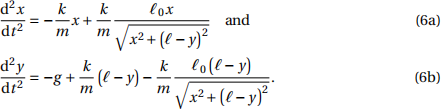
Hint: It is useful to get expressions for sinθ and cos θ in terms of the length of the spring (note this is not, in general!) and use θ as an intermediary variable.
![]() 3.2. Take! as a length scale and 4!/g as a time scale and non-dimensionalise the equations you found in the previous question (see appendix Afor a simpler example). Here we will define a non-dimensional parameter in our equations,
3.2. Take! as a length scale and 4!/g as a time scale and non-dimensionalise the equations you found in the previous question (see appendix Afor a simpler example). Here we will define a non-dimensional parameter in our equations,

Your solution should only contain x, y, their time derivatives (non-dimensionalised, that is; you can drop the primes once you’ve done it, since you will not use dimensional units after this), and σ .
Hint: The relation !0 = ! (1 ¡ σ), which you should justify, maybe useful.
3.3. Adapt one of the codes you have at your disposal (could be code for the non-linear pendu- lum, or the Rössler or Lorenz attractors) to solve the non-dimensionalised spring pendulum numerically. This time, make sure to keep the solve_ivp function that we discussed ear- lier with at least rtol=1e-5. (The smaller rtol, the smoother the picture but the longer it takes for the code to run.) If useful, you may start from the starter code springpendulum.py, replacing all the ![]() ???
???![]() with appropriate code.
with appropriate code.
Set the initial conditions to x0 = y0 = 1 and ![]() 0 = y(˙)0 = 0, and use σ = 1/4. Integrate the system for a total duration tend = 50.0, and when you run the code you should reproduce figure3, or at least the solution that is being displayed (cosmetic details are up to you). Seek help if you cannot reproduce figure 3!
0 = y(˙)0 = 0, and use σ = 1/4. Integrate the system for a total duration tend = 50.0, and when you run the code you should reproduce figure3, or at least the solution that is being displayed (cosmetic details are up to you). Seek help if you cannot reproduce figure 3!
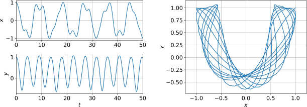
Figure 3: The spring pendulum solution for x0 = y0 = 1, ![]() 0 = y(˙)0 = 0, for 200 steps, and tend = 50.0.
0 = y(˙)0 = 0, for 200 steps, and tend = 50.0.
3.4. σ is a non-dimensional parameter in our equations, what does it measure about the system? What should we expect if we set σ to be very small? Set σ to be 0.0001, then use x0 = 0.8, y0 = 0.4, and ![]() 0 = y(˙)0 = 0. What happens? Why should this only happen for σ << 1?
0 = y(˙)0 = 0. What happens? Why should this only happen for σ << 1?
3.5. The state of a dynamical system at a given moment can be completely characterized by a point in phase space. In this case, phase space is four dimensional and spans x, y, ![]() , and y(˙) . Furthermore, because this system is neither damped, nor driven, the solution is constrained to lie on surfaces of constant energy.
, and y(˙) . Furthermore, because this system is neither damped, nor driven, the solution is constrained to lie on surfaces of constant energy.
Derive an expression for the non-dimensional energy in a spring pendulum using the non- dimensionalisation we used in part 3.2..
3.6. As a four dimensional space is difficult to imagine, we can gain some insight into the dy- namics of the spring pendulum system using a Poincaré section which is a two dimensional slice through a higher dimensional phase space. We create a point each time the trajectory intersects with our surface.
For example, in class, for the DDP, we had a three-dimensional phase space (θ, θ(˙), !ft) and took (θ, θ(˙)) sections along the !ftaxis. Other combinations could have been valid choices for Poincaré sections, for example, (θ, !ft) sections along the θ(˙) axis. In this final question, we will record the motion everytime the phase trajectory crosses a (y = 0,y(˙) > 0) state.
In a periodic system the motion repeats itself after a certain amount of time so the Poincaré section is made up of a lot less points.
If there is more than one frequency in the system and they are not commensurate, then the system will never repeat exactly. In this case the system is constrained to lie on a closed torus of phase space and a Poincaré section will become a slice of a torus. This means that the set of points in a Poincaré section will become a closed curve.![]()
Finally, the system may not be constrained by its dynamics to lie on any surface and so the whole phase space will be traversed. In this case the system is in a fully chaotic state.
In class, we could easily identify points on the !ftaxis because that’s the axis along which the time-integration proceeded. Here, on the other hand, the solution does not necessarily have y = 0 exactly at some, or any, time step. What it does have is a set of successive values for y that straddle zero. What you need to do to find a better estimate of the crossing is therefore to interpolate between the values that straddle zero in the right direction.
In the script find_roots .py, we give an example that will find the zeros of x = sin(t), with a time array that does not exactly contain values t = nπ . To find the zeros of x, it detects the places where two successive values of x change sign in the ascending direction (i.e., it finds the values of i for which xi < 0 and xi+1 > 0), and interpolates t (meant to approximate arcsin x) between the surrounding values to find an accurate version of the corresponding root of sin(t).
Once you have the times tr for which y(tr ) = 0,y(˙)(tr ) > 0, you can use other interpolations of
x and ![]() at times tr to create the values to display on your Poincaré section.1
at times tr to create the values to display on your Poincaré section.1
Combine find_roots .py and your code from part3.3. to plot a Poincaré section of (x, ![]() ) when y(˙) > 0, y = 0. As during the lecture, you also want to plot them as small dots rather than jointed lines, as in
) when y(˙) > 0, y = 0. As during the lecture, you also want to plot them as small dots rather than jointed lines, as in
plt.plot(xPoincare, dotxPoincare, ' . ' , markersize=0.5)
You will also want to run them for longer than the previous examples to start seeing some- thing.
Finally, we noticed that the default Runge-Kutta integration scheme implemented by solve_ivp led to inaccurate plots, even for extremely low values of rtol. While these inaccuracies
were barely perceptible up until now, they add up over long integrations and become vis- ible in Poincaré sections. Instead, we found that the Radau method gave the best results. (Here for example, we know that in the first case below, Poincaré sections must line up along closed trajectories.) To use the Radau method, simply add it as an option at the end of the solve_ivpcall, like this:
solution = solve_ivp( ... , rtol=1e-6 , method="Radau")
were “ ...” is a placeholder for the other inputs of the call. You could also consider lowering the relative tolerance, but the Radau method is slow as it is, and we don’t require you to be very precise.
(a) Set σ = 1/4, E = 1.0 and x0 = −0.75, ![]() 0 = 1.0, y0 = 0.20 (you need to figure out y(˙)0 on your own, but hint: checkout part3.5.). Now run your code and examine your Poincaré section.
0 = 1.0, y0 = 0.20 (you need to figure out y(˙)0 on your own, but hint: checkout part3.5.). Now run your code and examine your Poincaré section.
(b) Now repeat this but set E = 1.0 and x0 = −0.1, ![]() 0 = 1.0, y0 = 0.0.
0 = 1.0, y0 = 0.0.
Can you describe the difference in the dynamics in these 2 cases?![]()
A Non-dimensionalising equations
The dimensional equation for the non-linear pendulum is

To obtain eqn. (1), we modifiedit so that the quantities in them are non-dimensional. This means that we are going to define new units (and choose these units intelligently) then cast our equation into these units.
This is advantageous for two reasons:
• it will simplify our equations, and it will mean that we don’t need to pick our parameters (g and {) before we run the simulation, and
• it will make explicit the fact that what matters in a problem is often not the absolute value of parameters, but how they vary with respect to one another.
For example, in the pendulum problem (eq.8), if both the acceleration due to gravity and the length of the pendulum are doubled, the behaviour of the system remains the same. While this might seem obvious in this case, in larger, more complex sets of equations, non-dimensionalisation can be a great help.
To non-dimensionalise eq. (8) we need to pick new scales that are relevant to the problem. Nor- mally this would mean picking new scales for all dependent and independent variables (θ and t) however, in this case, θ is already non-dimensional so we can leave that alone. On the other hand, t has units of seconds and so we need to pick a scale for that quantity. For our timescale we will pick the period of the simple pendulum2 : τ =‘{/g (check yourself, the units of τ are seconds). In many problems there are several timescales at play and while we can technically pick any timescale, there are often very good reasons for picking one over another.
To convert an individual quantity into non-dimensional terms, we simply factor a τ out of it. We will then say that t = τtl where a prime indicates that the quantity is non-dimensional. Since θ doesn’t have units, θ = θl.
If we apply our non-dimensionalisation, eq. (8) becomes

which is completely free of any dimensional units.
Now we can run a simulation of the pendulum without having to worry about specifically what g and { are, then rescale time once the simulation is done with whichever g and { we choose.
This brings up one final advantage to non-dimensionalisation which applies specifically to simu- lating these systems numerically. If we simulate a pendulum that is 10 meters long in a gravitational acceleration of 9.8 m s¡2, this will yield a period of approximately 20 s (using the small angle ap- proximation). In this case, a time step of 0.5 s seems appropriate since that gives 40 time steps per period, which will probably be enough to resolve the motion of the pendulum over one period.
If we now want to simulate a pendulum that is 1 mm long on a missile that is accelerating at 300 m s¡2, the 0.5 s time step we used previously is nowhere near small enough to resolve the motion whose period is approximately 0.01 s. A time step of 0.5 s is 50 times larger than the period of the pendulum, and so is unable to resolve the motion at all.
The issue is that the time step is dependent on the physics, not on the mathematics.
If we non-dimensionalise the equations then the time step is in units of pendulum period (say 20 time steps per τ) so if the physics of the problem changes, the numerics of the problem don’t.
We are now going to derive a non-dimensional energy for the pendulum. We will start by writing the energy in dimensional form. If we set the origin of the system to beat the equilibrium point of the pendulum my dimensional energy is

In order to non-dimensionalise energy we need to pick a length scale L and a mass scale M. The obvious choices for these are the length and mass of the pendulum. Putting these into eq. (10) (and making sure to non-dimensionalise the E) we get

2023-12-13