COMP4041-LDO Linear and Discrete Optimization
Hello, dear friend, you can consult us at any time if you have any questions, add WeChat: daixieit
COMP4041-LDO Linear and Discrete Optimization
Coursework – Autumn Semester, Session 2023-2024
INSTRUCTIONS
This coursework is worth 70% of the overall module assessment, 50% is allocated to the submission of files as explained below and 20% is allocated to an open book online test in Moodle about the coursework.
The electronic submission via Moodle consists of the following files (please upload separate files, not compressed files):
1. One Excel file for the spreadsheet model, please name the file cw-cr-ID replacing ID with your own 8-digit student ID.
2. One LP-Solve file for the algebraic model, please name the file cw-cr-ID replacing ID with you own 8-digit student ID.
3. One demonstration video presenting your final optimization models, please name the file cw-cr-ID replacing ID with you own 8-digit student ID.
The normal submission deadline is 09 January 2024 at 15:00 hrs. If submitting after this date, a penalty of 5 marks (the standard 5% absolute) out of the 100 marks available will be applied for each late working day.
The late submission deadline is 16 January 2023 at 15:00 hrs. Submissions after this date will only be accepted if supported through the extenuating circumstances procedure, https://www.nottingham.ac.uk/studentservices/services/extenuating-circumstances.aspx.
The date/time for the test is Friday 12 January 2024 at 15:00-16:00 hrs. It is not a requisite to submit the coursework files for taking the test. Even if the coursework is submitted late or not submitted at all, the test can be taken on the specified date/time.
The coursework test will follow a similar approach as the workshop tests in the module. Some questions will be about your understanding of the submitted coursework and some questions will be about modifications to the problem and/or model. Questions in the test might also ask to submit a labelled screenshot of your model(s) before/after the required modifications. The questions could refer to any of the topics covered in the module but answers will be required for your submitted coursework.
Students should ensure that they have good Internet access to Moodle for taking the online coursework test. If a student anticipates problems with taking the coursework test at the specified date/time, they should get advice in advance from the module convenor.
Students are reminded of the University’s Advice on Academic Integrity and Misconduct and so they should adhere to this policy when completing this coursework and taking the open book test in Moodle. Student are expected to adhere to the University’s Policy on Academic Misconduct.
COURSEWORK DESCRIPTION
Refer to the Car Rental 1 and Car Rental 2 optimization problems described in sections 12.25 and 12.26 of the following book in the reading list:
Model Building in Mathematical Programming. H.P. Williams, Wiley, 5th edition, 2013.
Hard copies of the above book are available from the University libraries, but electronic copies of the relevant chapters are made available in Moodle.
The optimization models for these problems are given in sections 13.25 and 13.26, while the optimal solutions are described in sections 14.25 and 14.26 respectively. Study the descriptions, optimization models and optimal solutions for these problems to make sure you understand them well. In what follows, Car Rental refers to the integrated problem, that is, the model for Car Rental 1 then extended from Car Rental 2.
Develop an Excel spreadsheet model to solve the Car Retal optimization problem. The spreadsheet model should execute with no errors, even if the model is not complete or does not produce the correct optimal solution. Make sure to include appropriate labels and comments in the spreadsheet model to clarify the approach. Also include annotations and comments in the spreadsheet model to clearly illustrate the corresponding algebraic model being implemented, whether it follows the model given in the book or not. Good principles of spreadsheet modelling should be followed whenever possible.
Develop an LP-Solve model to solve the Car Rental optimization problem. The LP-Solve model should execute with no errors, even if the model is not complete or does not produce the correct optimal solution. Make sure to include appropriate comments in the LP-Solve model to clarify the algebraic formulation. Also include the algebraic compact notation as comments in the LP-Solve model to clearly illustrate the correspondence between each algebraic expression and the constraints implemented in the LP-Solve model. Explain the correspondence of your LP-Solve model to the algebraic model provided in the book and to the Excel spreadsheet model.
Develop a short demonstration video of maximum 15 minutes duration that describes the design and use of your spreadsheet model, the implementation of the LP-Solve model as well as the correspondence between the two models. The demonstration video should clearly explain in a logical and coherent way, the implementation of the spreadsheet and LP-Solve models with references to the algebraic model. The video should also describe how the spreadsheet model was designed (layout, calculations, solver settings, etc.) and how it can be used to understand the solution found. The video may also describe any issues, additional insights, reflections, and clarifications about your work. There is no need to describe the given optimization problem but references to it and the LP-Solve algebraic model might be needed. It is required that you appear in the video and holding your student ID card, even if for only a few seconds at the beginning, this is to confirm your identity as the person presenting the video. Any appropriate software may be used for producing the video, but please make sure the video file can be played in standard media players and/or Internet browsers. Also, please aim to keep the size of the file as small as possible while still ensuring good viewing quality. The maximum file size allowed for the video is 150MB. Make sure to select in advance suitable software to record your video without exceeding the maximum file size.
MARKING CRITERIA FOR COURSEWORK SUBMISSION
The purpose of this coursework is to assess your ability to understand and interpret an optimization problem and to implement the corresponding optimization model. If there is any element of the problem that is not entirely clear to you, please attempt to interpret such element in the best way you can and explain your rationale in the demonstration video. The given algebraic model for the problem might not be described in full detail and hence you will have to achieve an understanding of the model. If your optimization model or optimal solution do not correspond to the ones given in the book, then please explain as appropriate. Although you should endeavour to provide the correct model, this does not mean that all marks will be lost because of your model not finding the correct optimal solution. Marks are awarded for correctness but also for quality of the work as follows:
Correct Spreadsheet Model (30 marks): this refers to the spreadsheet model being fully correct in terms of modelling and solving the optimization problem, any innovative modelling mechanisms implemented, and the correspondence to the LP-Solve model.
Quality of Spreadsheet Model (20 marks): this refers to layout and presentation of the spreadsheet model for clarity and usability, any additional features developed to enhance the visualisation of the model and the solution, any additional features developed to enhance the implementation and usability of the model.
Correct and Clear LP-Solve Model (20 marks): this refers to the LP-solve model being fully correct and clear in terms of modelling, the lp-solve model solving the optimization problem correctly, and the correspondence to the spreadsheet model.
Quality of Demonstration Video (30 marks): this refers to the effectiveness and the visual quality of the video in explaining the optimization models, the optimal solutions obtained, any issues/insights/reflections that enhance the demonstration, video following the given guidelines.
IMPORTANT: Please note that since the reference optimization model and optimal solution are already provided, not questions will be asked about the interpretation or understanding of the problem, the reference model, or the reference optimal solution. If you think there is any error in the book sections provided, you are welcome to implement fixes and describe them in your demonstration video.
Use the actual demands that resulted from the prices you set in period 1 to rerun the model at the beginning of period 2 to set price levels for period 2 and provisional price levels for period 3.
Repeat this procedure with a rerun at the beginning of period 3. Give the final operational solution.
Contrast this solution to one obtained at the beginning of period 1 by pricing to maximise yield based on expected demands.
12.25 Car rental 1
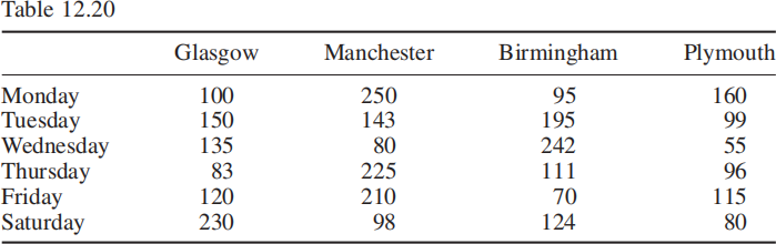
A small (‘cut price’) car rental company, renting one type of car, has depots in Glasgow, Manchester, Birmingham and Plymouth. There is an estimated demand for each day of the week except Sunday when the company is closed. These estimates are given in Table 12.20. It is not necessary to meet all demand.
Cars can be rented for one, two or three days and returned to either the depot from which rented or another depot at the start of the next morning. For example, a 2-day rental on Thursday means that the car has to be returned on Saturday morning; a 3-day rental on Friday means that the car has to be returned on Tuesday morning. A 1-day rental on Saturday means that the car has to be returned on Monday morning and a 2-day rental on Tuesday morning.
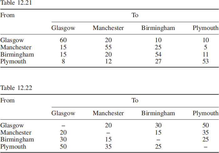
The rental period is independent of the origin and destination. From past data, the company knows the distribution of rental periods: 55% of cars are hired for one day, 20% for two days and 25% for three days. The current estimates of percentages of cars hired from each depot and returned to a given depot (independent of day) are given in Table 12.21.
The marginal cost, to the company, of renting out a car (‘wear and tear’, administration etc.) is estimated as follows:
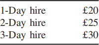
The ‘opportunity cost’ (interest on capital, storage, servicing, etc.) of owning a car is £15 per week.
It is possible to transfer undamaged cars from one depot to another depot, irrespective of distance. Cars cannot be rented out during the day in which they are transferred. The costs (£), per car, of transfer are given in Table 12.22.
Ten percent of cars returned by customers are damaged. When this happens, the customer is charged an excess of £100 (irrespective of the amount of damage that the company completely covers by its insurance). In addition, the car has to be transferred to a repair depot, where it will be repaired the following day. The cost of transferring a damaged car is the same as transferring an undamaged one (except when the repair depot is the current depot, when it is zero). Again the transfer of a damaged car takes a day, unless it is already at a repair depot. Having arrived at a repair depot, all types of repair (or replacement) take a day.
Only two of the depots have repair capacity. These are (cars/day) as follows:

Having been repaired, the car is available for rental at the depot the next day or may be transferred to another depot (taking a day). Thus, a car that is returned damaged on a Wednesday morning is transferred to a repair depot (if not the current depot) during Wednesday, repaired on Thursday and is available for hire at the repair depot on Friday morning.
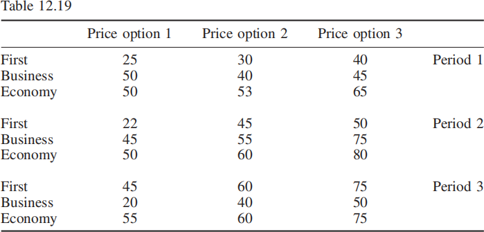
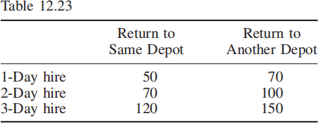
The rental price depends on the number of days for which the car is hired and whether it is returned to the same depot or not. The prices are given in Table 12.23 (in £).
There is a discount of £20 for hiring on a Saturday so long as the car is returned on Monday morning. This is regarded as a 1-day hire.
For simplicity, we assume the following at the beginning of each day:
1. Customers return cars that are due that day
2. Damaged cars are sent to the repair depot
3. Cars that were transferred from other depots arrive
4. Transfers are sent out
5. Cars are rented out
6. If it is a repair depot, then the repaired cars are available for rental.
In order to maximise weekly profit, the company wants a ‘steady state’ solu-tion in which the same expected number will be located at the same depot on the same day of subsequent weeks.
How many cars should the company own and where should they be located at the start of each day?
This is a case where the integrality of the cars is not worth modelling. Rounded fractional solutions are acceptable
12.26 Car rental 2
In the light of the solution to the problem stated in Section 12.25, the company wants to consider where it might be most worthwhile to expand repair capacity. The weekly fixed costs, given below, include interest payments on the necessary loans for expansion.
The options are as follows:
1. Expand repair capacity at Birmingham by 5 cars per day at a fixed cost per week of £18 000.
2. Further expand repair capacity at Birmingham by 5 cars per day at a fixed cost per week of £8000.
3. Expand repair capacity at Manchester by 5 cars per day at a fixed cost per week of £20 000.
4. Further expand repair capacity at Manchester by 5 cars per day at a fixed cost per week of £5000.
5. Create repair capacity at Plymouth of 5 cars per day at a fixed cost per week of £19 000.
If any of these options is chosen, it must be carried out in its entirety, that is, there can be no partial expansion. Also, a further expansion at a depot can be carried out only if the first expansion is also carried out, so for example option (2) at Birmingham cannot be chosen unless option (1) is also chosen. If option (2) is chosen, thereby also choosing option (1), these count as two options. Similar stipulations apply regarding the expansions at Manchester. At most three of the options can be carried out.
12.27 Lost baggage distribution
A small company with six vans has a contract with a number of airlines to pick up lost or delayed baggage, belonging to customers in the London area, from Heathrow airport at 6 p.m. each evening. The contract stipulates that each customer must have their baggage delivered by 8 p.m. The company requires a model, which they can solve quickly each evening, to advise them what is the minimum number of vans they need to use and to which customers each van should deliver and in what order. There is no practical capacity limitation on each van. All baggage that needs to be delivered in a two-hour period can be accommodated in a van. Having ascertained the minimum number of vans needed, a solution is then sought, which minimises the maximum time taken by any van.
On a particular evening, the places where deliveries need to be made and the times to travel between them (in minutes) are given in Table 12.24. No allowance
Up to six planes can be flown:
n ≤ 6.
13.24.3 Objective

(measuring in £1000) where Qi is the probability of scenario i.
This model has 1200 constraints, one bound and 982 variables, of which 117 are 0–1 integer and one general integer.
In defining the data, it is desirable that the demands in the scenarios cover the extremes as well as the most likely cases. The recommended sales will not exceed those of the most extreme scenario in the solution to this model. In this example, it can be seen that final demands (known with hindsight) exceed those of all scenarios in a few cases. As a result, the solution will not result in sales to meet all of these demands.
Models for subsequent weeks (with recourse) are obtained from this model by fixing prices and sales for weeks that have elapsed.
13.25 Car rental 1
We model this problem as a deterministic linear programme. There would be advantage to be gained from modelling it as a stochastic programme. In order to do this, we would need to obtain data to quantify the uncertain demand.
13.25.1 Indices
i, j = Glasgow, Manchester, Birmingham, Plymouth
t = Monday, Tuesday, Wednesday, Thursday, Friday, Saturday
k = 1, 2, 3 (days hired)
Although this is a ‘dynamic’ problem, we seek a steady-state solution and can therefore regard the set of days as ‘circular’, that is, Monday of a week ‘follows’ after the subsequent Saturday; that is, if t = Monday then t − 1 = Saturday.
13.25.2 Given data
Dit = estimated rental demand at depot i on day t as given in Table 12.19
Pij = proportion of cars rented at depot i to be returned to depot j as given in Table 12.21
Cij = cost of transfer of a car from depot i to depot j as given in Table 12.22
Qk = proportion of cars hired for k days
Ri = repair capacity of depot i
RCAk = rental cost for k days with return to same depot as given in Table 12.23
RCBk = rental cost for k days with return to another depot as given in Table 12.23
RCC = rental cost for Saturday with return to same depot on Monday
RCD = rental cost for Saturday with return to another depot on Monday
CSk = marginal cost to company of k day hire of a car for all i, t
13.25.3 Variables
n = total number of cars owned
nuit = number of undamaged cars at depot i at the beginning of day t for all i, t
ndit = number of damaged cars at depot i at the beginning of day t for all i, t
trit = number of cars rented out from depot i at beginning of day t for all i, t
euit = undamaged cars left at depot i during day t for all i, t
edit = damaged cars left at depot i at the beginning of day t for all i, t
tuijt = number of undamaged cars at depot i at the beginning of day t, to be transferred to depot j for all i, j, t
tdijt = number of damaged cars at depot i at the beginning of day t, transferred to depot t for all i, j, t
rpit = number of damaged cars to be repaired at depot i on day for all i, t
2023-12-12