Econ 140B Final Exam Practice Exam 2
Hello, dear friend, you can consult us at any time if you have any questions, add WeChat: daixieit
Econ 140B Final Exam
Practice Exam 2
1 Short Answer & Multiple Choice
(a) Which is the correct interpretation for the coefficient estimate for x1 in the logistic regression below? (Circle all that apply.)
Call:
glm(formula = Y ~ x1 + x2, family = "binomial")
Coefficients:
Estimate Std . Error z value Pr(>|z|)
(Intercept) 0.1 0.2 0.5 0.6
x1 2.3 0.4 5.8 7e-09 ***
x2 -2.7 0.4 -6.6 3e-11 ***
---
Signif . codes: 0 ‘***’ 0.001 ‘**’ 0.01 ‘*’ 0.05 ‘.’ 0.1 ‘ ’ 1
(Dispersion parameter for binomial family taken to be 1)
Null deviance: 276.76 on 199 degrees of freedom
Residual deviance: 113.34 on 197 degrees of freedom
AIC: 119.3
Number of Fisher Scoring iterations: 6
(i) log(r[Y = 1]) increases 2.3 units for a one unit increase in x1.
(ii) log (r[Y = 1]\r[Y = 0])increases tenfold for a one unit increase in x1.
(iii) The odds of Y = 1 increase tenfold for a one unit increase in x1.
(iv) Y increases 2.3% for a one unit increase in x1.
(v) (i) and (iii) are both correct.
(vi) (ii) and (iv) are both correct.
(b) Give a brief explanation of what a “partial effect” is in the context of logistic regression.
(c) In the logistic regression in part (a), the mean of x1 is zero and the mean of x2 is also zero. Compute the partial effect of x2 on Y at the sample average.
Solution. The predicted probability is eb0 /(1 + eb0 ) ≈ 1/2 so the partial effect is (1/2) × (1 − 1/2) × (−2.7) ≈ −0.675.
2 Logistic Regression – Credit Card Applications
A credit card company has asked us to build a decision rule for accepting or rejecting future credit card applications. For 1,312 past applications, we have the actual outcome and seven applicant characteristics. Thee outcome of interest is the binary variable given.card indicating if the appli- cation for a credit card was accepted or not. Of the 1,312 applicants, 1,017 (or 78%) were given a card, 295 were denied. The seven characteristics consist of four binary and three continuous variables:
home.owner = {0,1}. Does the individual own his or her home?
self.employed = {0,1}. Is the individual self-employed?
has.negative.reports = {0,1}. Does the individual have any bad credit reports?
have.card.already = {0,1}. Does the individual have any major credit cards already? age = Age in years
annual.income = Yearly income (in USD 10,000)
ratio.spending.income = Ratio of monthly credit card expenditure to yearly income
We will build a classifier using logistic regression on a training subsample of the data and test it on a held-out validation sample. For training, 500 of the 1312 applications are randomly selected, leaving the remaining 812 for testing.
(a) In our current context, what are the two types of errors that a classifier can make?
In the present decision-making context, which type of mistake do you think is “worse” and why? (Full credit for good reasoning; either error can be the correct answer.)
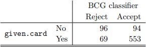
(b) This credit card company previously hired Bad Consulting Group, Inc to develop a decision rule. These consultants came up with the rule to reject applicants if they have bad credit reports (has.negative.reports = 1) and accept all others (has.negative.reports = 0). In the testing sample of 812 applicants, this decision rule gives the following results:![]()
We will try to build a better rule by using data. Consider the below stepwise selection commands and (excerpted) output and the summary of the final model.
> base <- glm(given.card ~ 1, family=binomial, data=CreditCard[training.samples,])
> full <- glm(given.card ~ has.negative.reports + have.card.already + home.owner + self.employed +
age + annual.income + log(ratio.spending.income), family=binomial, data=CreditCard[training.samples,])
> final <- step(base, scope=formula(full), direction="forward", k=log(length(training.samples))) Start: AIC=520.17
given.card ~ 1
Step: AIC=88.65
given.card ~ log(ratio.spending.income)
Step: AIC=83.08
given.card ~ log(ratio.spending.income) + annual.income
Step: AIC=78.7
given.card ~ log(ratio.spending.income) + annual.income + has.negative.reports
> summary(final)
Call:
glm(formula = given.card ~ log(ratio.spending.income) + annual.income + has.negative.reports, family=binomial)
Coefficients:
Estimate Std . Error z value Pr(>|z|)
(Intercept) 23.1706 6.4622 3.586 0.000336 ***
log(ratio.spending.income) 3.5677 0.9277 3.846 0.000120 ***
annual.income 0.8466 0.2701 3.135 0.001719 **
has.negative.reportsTRUE -3.9433 2.0295 -1.943 0.052017 .
(c) Give a precise and numerical explanation of what these results say about the relationship between ratio.spending.income and the outcome given.card.
(d) Based on this output, how much more likely or less likely to be given a credit card, relative to not given a card, is someone with prior negative reports compared to someone without prior negative reports?
Solution. e −3.9433 times less likely, relative to not being given a card.
(e) We obtain from the final selected model (in the above summary) estimated probabilities
for giving each of the 812 testing applicants a credit card, that is we find the estimated
r[given.card = 1 | X],for X = (ratio.spending.income, annual.income, has.negative.reports). Our decision rule will be to accept applications when this probability is above a cut-off κ .
For κ = {0.15, 0.25, 0.35}, this rule gives the following results:
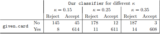
(i) For the first type of error you identified in part (a), examine how this error responds to changes in κ, and give a well-reasoned explanation for any pattern you find.
(ii) Based on this output and your answer in part (a), what is your preferred choice of κ and why? (Improving on the BCG classifier is not a good reason why!)
3 Transformations
The following questions pertain to a regression model fit, summarized below, to data on the brain weight (brain.weight, in grams) and the body weight (body.weight, in kilograms) of 62 mammals.
Call:
lm(formula = log(brain.weight) ~ log(body.weight))
Residuals:
Min 1Q Median 3Q Max
-1.71550 -0.49228 -0.06162 0.43597 1.94829
Coefficients:
Estimate Std . Error t value Pr(>|t|)
(Intercept) 2.13479 0.09604 22.23 <2e-16 ***
log(body.weight) 0.75169 0.02846 26.41 <2e-16 ***
---
Signif . codes: 0 ‘***’ 0.001 ‘**’ 0.01 ‘*’ 0.05 ‘.’ 0.1 ‘ ’ 1
Residual standard error: 0.6943 on 60 degrees of freedom
Multiple R-squared: 0.9208, Adjusted R-squared: 0.9195
F-statistic: 697.4 on 1 and 60 DF, p-value: < 2.2e-16
(a) How does the model assume brain weight and body weight are related in their original scale?
(b) How would you justify using the log transform here? What additional evidence, if any, would you like to base your decision on?
(c) What percentage of the variation in the response is explained by regressing onto the explana- tory variable? Do we have reason to believe in a linear relationship between these variables? State the formal hypothesis test (and the conclusions).
(d) What would the model predict for brain weight for a mammal with a body weight of 110 kgs? If sfit(log 110) = 0.145 (in units of log grams), give a 95% predictive interval for the brain weight.
4 Model Building
This problem examines predicting wages based on observed characteristics. The data consists of 550 employed individuals in 1978 and has the following variables: log of hourly wage (log.wage), years of labor market experience (exper and its square exper2), years of education (educ), age, number of dependent kids (coded as 0, 1, 2, or ≥ 3), and binary variables for sex (Male or Female), race (White or Nonwhite), married (Yes or No), and being a union.member (Yes or No).
(a) Consider the below sequence of progressively more complicated models.
Model 1: log.wage ~ exper + educ + sex
Model 2: log.wage ~ exper + exper2 + educ + sex
Model 3: log.wage ~ exper + exper2 + educ + sex + race + married + age + kids
Model 4: log.wage ~ exper + exper2 + educ + sex + race + married + age + kids + union.member Model 5: log.wage ~ exper + exper2 + educ + sex + race + married + age + kids + union.member
+ sex * race
Model 6: log.wage ~ exper + exper2 + educ + sex + race + married + age + kids + union.member + sex * race + union.member * educ
For this sequence of models we have the following results:
Analysis of Variance Table
Res.Df RSS Df Sum of Sq F Pr(>F)
Model 1 vs . Model 2 545 85.927 1 1.6118 11.1951 0.0008773 ***
Model 2 vs . Model 3 542 84.372 3 1.5549 3.6000 0.0134441 *
Model 3 vs . Model 4 541 79.475 1 4.8974 34.0160 9.43e-09 ***
Model 4 vs . Model 5 540 78.548 1 0.9274 6.4417 0.0114275 *
Model 5 vs . Model 6 539 77.601 1 0.9469 6.5768 0.0106014 *
(i) Briefly describe what is being presented in each row of the “Analysis of Variance Table” and what you conclude from the results of each row.
(ii) Briefly explain what is wrong with this approach to model building.
(b) Instead of the above, consider the following R commands and (excerpted) output from auto- mated method to build a model based on BIC.
> null <- lm(log.wage ~ 1, data=cps)
> full <- lm(log.wage ~ . + .^2, data=cps)
> fwdBIC.part_b <- step(null, scope=formula(full), direction="forward", k=log(n)) Start: AIC=-779.02
log.wage ~ 1
Step: AIC=-843.17
log.wage ~ sex
Step: AIC=-903.21
log.wage ~ sex + educ
Step: AIC=-985.57
log.wage ~ sex + educ + age
Step: AIC=-1011.71
log.wage ~ sex + educ + age + union.member
Step: AIC=-1013.29
log.wage ~ sex + educ + age + union.member + exper2
Step: AIC=-1015.49
log.wage ~ sex + educ + age + union.member + exper2 + educ:union.member
Step: AIC=-1016.83
log.wage ~ sex + educ + age + union.member + exper2 + race +
educ:union.member
(i) Briefly describe the process being used here to build a model.
(ii) Explicitly list the elements of this process which are controlled by the user as opposed to what is controlled by the computer.
(c) Next, consider a slightly altered version of the same process.
> model1 <- lm(log.wage ~ exper + educ + sex)
> full <- lm(log.wage ~ . + .^2, data=cps)
> fwdBIC.part_c <- step(model1, scope=formula(full), direction="forward", k=log(n)) Start: AIC=-985.57
log.wage ~ exper + educ + sex
Step: AIC=-1011.71
log.wage ~ exper + educ + sex + union.member
Step: AIC=-1013.29
log.wage ~ exper + educ + sex + union.member + exper2
Step: AIC=-1015.49
log.wage ~ exper + educ + sex + union.member + exper2 + educ:union.member
Step: AIC=-1016.83
log.wage ~ exper + educ + sex + union.member + exper2 + race +
educ:union.member
(i) Explain any differences between this approach and the one in part (b).
(ii) The final selected models contain different variables but the final BIC values are identical (it’s not rounding error). How do you explain this?
(iii) Comparing the two models of parts (b) and (c), which model do you prefer, and why?
(d) The data also contains indicators for job.type, grouped into 8 categories. These categories appear on the x-axis of the plot below.
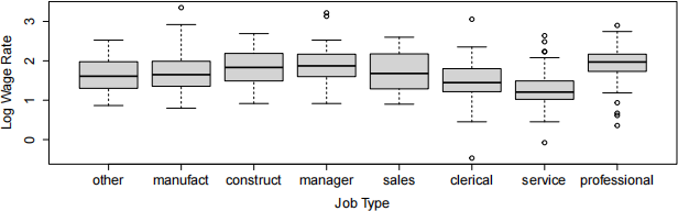
We also construct a new variable job.level that collapses job.type into three categors: LOW = {clerical, service}, MEDIUM = {other, manufact, sales}, and HIGH = {construct, manager, professional}.
Our goal is to select one of these two measures of job description to add to the final model selected in part (e). We have the following commands and output.
> reg.job.type <- lm(log.wage ~ exper + educ + sex + union.member
+ exper2 + race + educ:union.member + job.type)
> reg.job.level <- lm(log.wage ~ exper + educ + sex + union.member
+ exper2 + race + educ:union.member + job.level)
> c(extractAIC(reg.job.type, k=2)[2], extractAIC(reg.job.level, k=2)[2])
[1] -1079.569 -1076.706
> c(extractAIC(reg.job.type, k=log(n))[2], extractAIC(reg.job.level, k=log(n))[2]) [1] -1014.920 -1033.607
(i) Explain what is being computed in the final two lines and how to evaluate the numerical output.
(ii) Identify the models chosen by each method. Explain these choices, and why they are the same or different.
2023-12-10