AMATH 301 Rahman Coding Project 9
Hello, dear friend, you can consult us at any time if you have any questions, add WeChat: daixieit
AMATH 301 Rahman
Coding Project 9
Due Thursday, December 7th at 11:59pm
Problem 1
The FitzHugh-Nagumo model is a system of ordinary differential equations used to describe the excitation of a neuron membrane:
In this model, v(t) is the membrane voltage at time t and w(t) is a variable representing the activity of several types of membrane channel proteins. The function I(t) represents an external electrical current, and the parameters a, b and τ are constants controlling the channel protein activity.
In this problem, we will assume that a = 0.7, b = 1 and τ = 12 and that
Throughout this problem, we will assume that the initial voltage is 1 and the initial channel activity is 0.
That is,
v(0) = 1 and w(0) = 0.
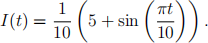
You should find that the voltage looks approximately like this:
Notice that this solution is roughly periodic. It is very important in neuroscience to be able to predict the firing rate of a neuron. The firing rate is
where the firing period is the distance between two adjacent peaks. In this problem, we will estimate the period by finding the distance between the first two peaks in our approximate solutions. From the diagram above, you can see that the firing period is roughly 45, and so the firing rate is roughly 1/45 ≈ 0.02.
Use ode45 (for MATLAB) or solve_ivp (for Python) to solve the system described above from time t = 0 to t = 100 with ∆t = 0.5. Save your approximations for the voltage at each time in a 201 × 1 column vector named A1.
Find the time when the voltage that you saved as A1 first reaches a maximum. (You can see from the diagram above that this time must be somewhere between 0 and 10.) Save this time in a variable named A2.
Find the time when the voltage reaches a the second peak. (You can see from the diagram above that this time must be somewhere between 40 and 50.) Save this time in a variable named A3.
Use your previous two answers to calculate the firing rate and save your answer in a variable named A4.
Problem 2
Consider Chua’s circuit
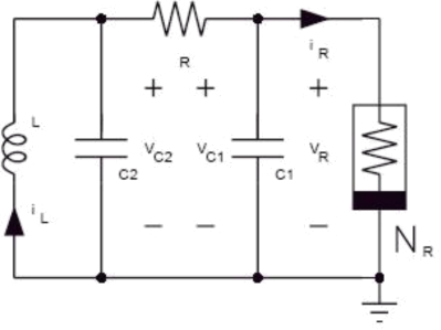
This circuit can be chaotic for the correct parameters. We can model this using Kirchoff’s laws. After nondimensionalizing the model, it simplifies to
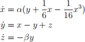 (1)
(1)
(1) Use ode45 (for MATLAB) or solve_ivp (for Python) to solve the system described above with parameters alpha = 16 and beta = 30, and initial condition x(0) = 0.1, y(0) = 0.2, z(0) = 0.3 from time t = 0 to t = 100 with ∆t = 0.05. First plot the phase space and comment on whether or not it is chaotic; if it is not chaotic save it as A5 = 0 and if it is chaotic save it as A5 = 1. Save your approximations for the entire solution at each time in a 3 × 2001 matrix named A6.
(2) Repeat the process with x(0) = 0.1, y(0) = 0.2 + 10−5 , z(0) = 0.3. Calculate the maximum difference in absolute value between A6 and the new solution. Since we have a matrix, you have to do max twice:
max(max(abs())) Save this value as A7.
(3) Repeat the process with beta = 100 and initial condition x(0) = 0.1, y(0) = 0.2, z(0) = 0.3. Plot the phase space and comment on whether or not it is chaotic; if it is not chaotic save it as A8 = 0 and if it is chaotic save it as A8 = 1.
Problem 3
Consider the boundary value problem

The true solution to this boundary value problem is
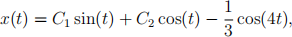
where
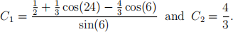
The solution looks like this:
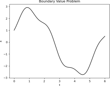
(1) Following the finite difference process we used in lecture, use a second order difference scheme to approximate ¨x and rewrite this initial value problem as a linear system of equations Ax = b. Use ∆t = 0.1. Note that there will be 61 total t-values, but we are only trying to approximate x at the interior times. The matrix A should be Nint × Nint, where Nint is the number of interior times, and the vector b should be Nint × 1. Save a copy of A in a variable named A9. Save a copy of b in a variable named A10.
Solve this linear system using Gaussian elimination (the backslash operator in MATLAB or the solve function in python). Make a 61×1 column vector containing the x values at all times (including the two boundary values) and save a copy of this vector in a variable named A11.
Find the maximum (in absolute value) error between this approximation and the true solution. Save this error in a variable named A12.
(2) Now solve the problem using the shooting method. Remember, you need to convert this second order ODE into a system of two first order ODEs. Apply a bisection scheme to the usual IVP solvers ode45 (MATLAB) or solve_ivp (Python) using ∆t = 0.1. For the second initial conditions, you can use the plot to help you test out values that will get you on different sides of the right boundary condition. Break out of the loop for bisection when the difference between your approximation at the right boundary point and the exact value at the right boundary point is less than 1e-8; i.e., |xapprox(6) − x(6)| = |xapprox(6) − 0.5| < 10−8 . Save the numerical solution as a 61 × 1 column vector A13 and the maximum (in absolute value) error max |xapprox − x| as A14. Further save the maximum difference in absolute value between the solution from part 1 and this solution as A15 = max(abs(A13 - A11)).
2023-12-09