1    Short Answer & Multiple Choice

(a) Which of the following statements are TRUE for logistic regression?  (Circle all that apply.)

(i)  The residuals are uncorrelated with the fitted values.

(ii)  The odds ratio is always above 1.

(iii)  The log odds ratio is always negative.

(iv)  Different regressions can be compared using BIC.

(v) All of the above statements are true.

(b) In the context of variable selection:

(i) Explain the difference between forward and backward stepwise selection.

(ii) Explain the difference between the BIC and AIC selection criteria.

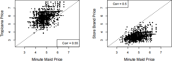
2    Linear Regression – Orange Juice Prices

We have 9649 observations of weekly orange juice prices and sales volume from different locations of a supermarket chain.  The data has the sales volume and price for Minute Maid orange juice (re- spectively minute.maid.sales in gallons and minute.maid.price in dollars per gallon), as well as the prices per gallon for Tropicana (tropicana.price) and the store brand (store.brand.price). We also have indicators for whether each brand was featured in the store’s marketing for that week (minute.maid.ad, tropicana.ad, and store.brand.ad, all binary indicators).

(a) Using the plots below, comment on the pricing strategy of each brand.  What position in the market does each brand occupy?  (“market position” can be defined as  “the place a brand occupies in consumers’ minds relative to competing offerings”.)

(b)  Describe the regression being run in the (abbreviated) output below.  In terms of Minute Maid sales and price, what does the slope coefficient represent?  Interpret the numerical value (both the sign and magnitude).

Call:

lm(formula  =  log(minute.maid.sales)  ~  log(minute.maid.price))

Coefficients:

Estimate  Std .  Error  t  value  Pr(>|t|)

(Intercept)                                5.33            0.16          33      <2e-16  ***

log(minute.maid.price)        -2.64              0.05          -54     <2e-16  ***

(c)  Consider the (abbreviated) regression output below. In terms of Minute Maid sales, what do the coefficients of log(tropicana.price) and log(store.brand.price) represent?  Inter- pret the numerical values (both the sign and magnitude).

Call:

lm(formula  =  log(minute.maid.sales)  ~  log(minute.maid.price)  +

log(tropicana.price)  +  log(store.brand.price))

Coefficients:

Estimate  Std .  Error  t  value  Pr(>|t|)

(Intercept)                                9.94            0.17            58     <2e-16  ***

log(minute.maid.price)        -4.15              0.05          -77     <2e-16  ***

log(tropicana.price)            1.60            0.06          28     <2e-16  ***

log(store.brand.price)          1.29              0.05          26     <2e-16  ***

(d)  Consider now the expanded model shown below.

Call:

lm(formula  =  log(minute.maid.sales)  ~  log(minute.maid.price)  *

minute.maid.ad  +  log(tropicana.price)  +  log(store.brand.price))

Coefficients:

Estimate  Std .  Error  t  value  Pr(>|t|)

(Intercept)                                                                    10.73            0.09         122      <2e-16  ***

log(minute.maid.price)                                              -3.14              0.06          -53     <2e-16  ***

minute.maid.adTRUE                                                        1.89             0.13            14      <2e-16  *** log(tropicana.price)                                                    0.98              0.05          18      <2e-16  *** log(store.brand.price)                                                1.10              0.04          24     <2e-16  *** log(minute.maid.price):minute.maid.adTRUE       -0.86            0.08         -10     <2e-16  ***

(i)  Give a precise interpretation of the coefficient estimate for minute.maid.adTRUE. Does this value make sense to you? Why or why not?

(ii) What does the coefficient estimate on log(minute.maid.price):minute.maid.adTRUE represent?  That is, visually, what would we learn from this estimate if the data were plotted? Does the estimate value make sense to you (both the sign and the magnitude)?

(e)  Consider the following R commands.

> model1  <-  lm(log(minute.maid.sales)  ~  log(minute.maid.price))

> model2  <-  lm(log(minute.maid.sales)  ~  log(minute.maid.price)  +  log(tropicana.price) +  log(store.brand.price))

> model3  <-  lm(log(minute.maid.sales)  ~  log(minute.maid.price)  +  log(tropicana.price) +  log(store.brand.price)  + minute.maid.ad)

> model4  <-  lm(log(minute.maid.sales)  ~  log(minute.maid.price)*minute.maid.ad

+  log(tropicana.price)  +  log(store.brand.price))

>  extractAIC(model1,k=log(length(minute.maid.sales)))

>  extractAIC(model2,k=log(length(minute.maid.sales)))

>  extractAIC(model3,k=log(length(minute.maid.sales)))

>  extractAIC(model4,k=log(length(minute.maid.sales)))

(i)  Explain in a few sentences what is being done here. What do the final four commands do and what do we learn about each regression model?

(ii)  The final four commands output the following

[1]         2.000    -8306.936

[1]            4.00  -10409.04

[1]            5.0    -12329.1

[1]            6.00  -12423.01

What do we conclude from this output?  Solution.  We  conclude  that  the fourth model is the  best,  according  to  the BIC criterion,  because  the  BIC value  is smallest  (closest to negative infinity) .

3    Classification & Model Building – Spam Filtering

Our goal for this question is to build an email spam filter:  based on observed  characteristics of an email message we want to build a classification rule for assigning the message either as spam (marked with a “1”) or not spam (“0”). To build our filter we have a data of 4601 emails, and for each message we have a human-assigned label spam (1 for spam, 0 for not spam) and the following characteristics:

•  caps_avg = the average of the lengths of strings of capital letters used in the email (e.g.  “The” = 1, “HELLO” = 5)

•  c_paren,  c_exclaim,  c_dollar = the percentage of characters in the message which are round or square parentheses, i.e.  “(”, “]”, “)”, or “]”, exclamation points, “!”, and dollar signs, “$”,respectively. (Percentages are between 0 and 100.)

(a) In our current context, what are the two types of errors that a classifier can make?

In the present context, is one type of mistake “worse” than the other? Explain your reasoning.

Use the following output to answer parts (b) – (f).

Call:

glm(formula  =  spam  ~  caps_avg  +  c_paren  +  c_exclaim  +  c_dollar,

family  =  "binomial",  data  =  spam)

Coefficients:

Estimate  Std .  Error  z  value  Pr(>|z|)

(Intercept)        -1.75              0.07          -25     <2e-16  ***

caps_avg               0.21             0.02            12      <2e-16  ***

c_paren              -1.66              0.23           -7       2e-13  ***

c_exclaim             1.38             0.11           12      <2e-16  ***

c_dollar              11.86              0.62            19      <2e-16  ***

Null  deviance:  6170.2    on  4600    degrees  of  freedom

Residual  deviance:  4160.7    on  4596    degrees  of  freedom

AIC:  4171

In addition to the variables defined above, we also have word counts for 43 different words, which are stored in variables like w_<word>.   For example w_credit is the number of times the word “credit” appears in the message.  We want to build a classifier that includes these word counts only if that word is relevant for predicting spam. We will take the train/test approach, holding out 1000 messages for testing.  We will choose variables using (i) forward stepwise selection based on AIC, (ii) on BIC, and (iii) selection using the LASSO.

(g)  Briefly explain in words the three approaches to model building, and how they differ from each other and what advantages and disadvantages they each have.

(i)  Stepwise AIC:

(ii)  Stepwise BIC:

(iii) LASSO:

On the 1000 held-out messages, we obtain predictions from each selected model and flag a message as spam if the estimated r[spam = 1|X] > 0.5 (just like part (f)).  For each of the three models, we then computed the following for each of the 1000 held-out messages:

error = spam − ✶{r[spam = 1|X] > 0.5}

where  ✶{r[spam = 1|X] > 0.5} indicates if the estimated r[spam = 1|X] > 0.5.  We obtained the following results.

(h)  Based on these results, which method of model selection do you prefer and why?  Refer to your answer in part (a).

4    Logistic Regression - Air Conditioning

For 546 homes we observe the following information

AC = 1 if it has air conditioning, 0 if not,

price = sale price, and

bedrooms = number of bedrooms.

Our goal is to predict which houses have air condition and which do not.

(a) First we use a logistic regression with only bedrooms and obtain the following output.

Call:

glm(formula  =  AC  ~  bedrooms,  family  =  "binomial")

Coefficients:

Estimate  Std .  Error  z  value        Pr(>|z|)

(Intercept)     -2.179           0.399     -5.46  0.000000047

bedrooms             0.469            0.127        3.68          0.00023

Give a precise, numerical interpretation of the relationship between bedrooms and AC by:

(i) Interpreting the coefficient estimate, 0.469, in this context.

(ii) Interpreting the statistical significance as best you can with this output.

(b) We now switch to using price and obtain the following output.

Call:

glm(formula  =  AC  ~  price,  family  =  "binomial")

Coefficients:

Estimate    Std .  Error  z  value                    Pr(>|z|)

(Intercept)  -3.76328283    0.34599029     -10.9  <0.0000000000000002

price               0.00004223    0.00000459         9.2  <0.0000000000000002

Based on this output, is price or bedrooms better at predicting whether or not a house has AC? Cite specific numeric evidence in favor or your argument.

Use the plot below to answer the next two questions.