STAT 404: Design and Analysis of Experiments FINAL EXAM, 2022
Hello, dear friend, you can consult us at any time if you have any questions, add WeChat: daixieit
STAT 404: Design and Analysis of Experiments
FINAL EXAM, 2022, Dec. 13, 3:30–6:00 pm
1. [6+1] We emphasize three design of experiment dogmas/principles in STAT 404: randomization, blocking and replication.
(a) [2 + 1] Name a design which employs blocking but does not have the word “blocking” in its name. A bonus mark if you can name two of them.
(b) [2] Randomization involves randomly assigning treatments to units. Describe another way to use randomization for analyzing a two-sample design/problem.
(c) [2] Name one thing that we cannot do in a full-factorial design without repli- cates. Describe what our suggested remedy to this is for data analysis.
2. [4] Name two diferences between the 2-level fractional factorial design and the 2- level full factorial design based on our discussions in this course. We accept any sensible suggestions, but be sure to use complete sentences. Beware that incorrect statements will be penalized even if the general ideas are correct.
3. [6] Under the standard linear model, the relationship between the response variable y and predictors/covariates x1 , . . . , xp are as follows:
y = β0 + x1 β1 + x2 β2 + · · · + xp βp + E .
The collected data are denoted as fyi , xi g, i = 1, . . . , n. We omit other details but highlight that (1) the predictors are not random and (2) the error term Ei are i.i.d. N(0, σ2 ). The least squares estimator of the regression coefficient vector (in matrix notation) is given by
β(ˆ) = (Xn(l)Xn )-1 Xn(l)yn.
If it helps, you may consider a concrete example with p = 2 and n = 4.
(a) [3] Suppose instead that the error distribution has mean 0 and variance σ2 but is not necessarily normal. Name a well-known property ofβ(ˆ) under the standard model that is no longer valid. Provide a brief explanation (not a proof).
(b) [3] Suppose that the values of the predictors x1 , . . . , xp are scaled by a factor of 2. Describe the efect of this scaling on β(ˆ) in the standard model. Provide a brief explanation.
4. [17] Three poisons (I, II, III) are randomly allocated to animals in four groups (A, B, C, D). Three animals in each group receive the same poison. The survival times of the animals are given in the following table.
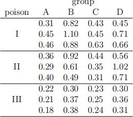
The code to load the data is provided in the ile Rcode2022final. txt on Canvas.
(a) [6] A sloppy professor regarded the design as a one-way layout with three treatments being the three poisons. Complete his ANOVA table. Not every cell needs to be flled.
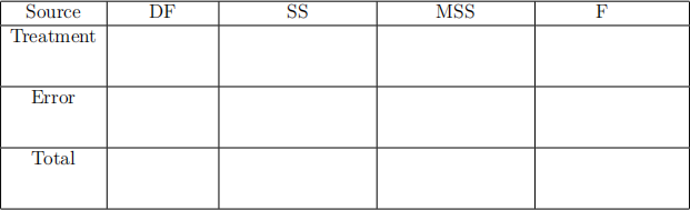
(b) [2] Determine whether he inds the treatment efect signiicant at the 5% level (under the wrong model).
(c) [6] Compute his simultaneous 95% CI’s for the three diferences in mean treat- ment efects using Tukey’s method (under the wrong model).
(d) [3] State if the MSS(err) value that he obtained is larger or smaller than the one he would obtain in the correct two-way layout. Provide a brief explanation. Do not compute the actual values.
5. [15] A 2-level fractional factorial design with 8 factors can be formed by either of the following two sets of deining relations:
(A) 6 = 124 ; 7 = 135 ; 8 = 245 .
(B) 6 = 125 ; 7 = 1235 ; 8 = 1245 .
(a) [6] Derive the deining contrasts subgroup of both designs.
(b) [2] Determine the resolutions of these two designs.
(c) [4] Determine the efects (main or interaction) confounded with the main efect of factor 2 in Design (B).
(d) [3] Suppose there are 4 replicates for each run. Calculate the degrees of freedom for SS(err).
6. [6] Consider a 2-level fractional factorial design with 6 treatment factors and 2 blocking factors. The deining relations are given by
6 = 124 ; B1 = 135 ; B2 = 245 .
(a) [3] State how many blocks this design has. Provide a brief explanation.
(b) [3] State how many runs there are in each block. Provide a brief explanation.
7. [28] In a door panel stamping experiment, 6 factors (each at 2 levels) were chosen and studied for their efects on the formality of a panel. One measure of formality is the thinning percentage of the stamped panel at a critical position.
The six factors are (A) concentration of lubricant, (B) panel thickness, (C) force on the outer portion of the panel, (D) force on the inner portion of the panel, (E) punch speed, and (F) thickness of lubrication.
The experiment was done over two days. “Day”was consider to be a blocking factor (G) to reduce the inluence of the day-to-day variation, with“-”representing day 1 and “+”day 2.
The experiment used a 27-2 resolution IV design with deining contrasts subgroup
I = ABCF = CDEG = ABDEF G .
We have k = 6, p = 1 and b = 1 in our notation. Yet, it is called 27-2 because G is regarded as a factor.
The code to load the design matrix and response y is provided in the ile Rcode2022final. txt on Canvas.
Note that the design is diferent from the one used in the assignment.
(a) [10] Derive the alias groups that contain a main factor.
(b) [4] Name all two-factor interactions that are not confounded with any other two-factor interactions.
(c) [6] The ile Rcode2022final. txt provides logit(y) values and some useful code. Compute efect estimates for A, B , C , AB , AC, and BC (6 efects). Do not consider other factors that are aliased with them if any.
(d) [4] Efect estimates for all alias groups are given in the ile Rcode2022final. txt. Identify the signiicant efects using a half-normal plot (based on your discretion). Write the itted model.
(e) [4] Describe the recommended factor settings for reducing/minimizing percent- age thinning.
8. [12] Jewelry appraisers recorded the clarity, the carat (a measure of mass), and the suggested prices (in hundreds of dollars) of several diamonds. The clarity grades range from 1 to 6 where higher-grade diamonds are more desirable.
Regard carat as a covariate, clarity as the treatments, and price as the response.
Note that the dataset difers from the one in the lab.
The code to load the data is provided in the ile Rcode2022final. txt on Canvas.
(a) [8] Complete the ANCOVA table. Not every cell needs to be flled.
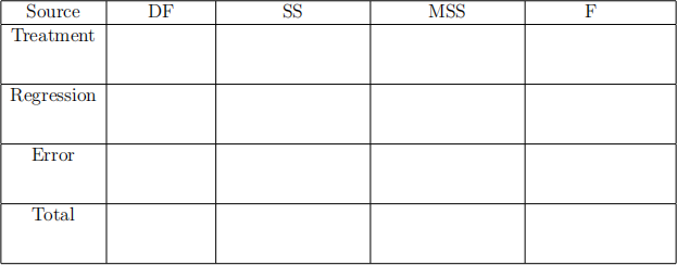
(b) [4] Construct a 95% two-sided conidence interval for the error variance σ 2 . Remark: you have the knowledge to work on this problem though this was not directly discussed in this course.
9. [6] The model for analysis of covariance is postulated as
yij = η + τi + β(xij - ![]() ·· ) + Eij
·· ) + Eij
with Eij being i.i.d. N(0, σ2 ). The covariate x is regarded as non-random. We consider a scalar x and omit other model details here.
We estimate the i-th treatment mean by
ˆ(τ)i = ![]() i· -
i· - ![]() ·· - β(ˆ)(
·· - β(ˆ)(![]() i· -
i· - ![]() ·· )
·· )
with estimated regression coefficient

(a) [3] Prove that Cov(![]() i· , β(ˆ))
i· , β(ˆ))
(b) [3] Show that in general, Cov(ˆ(τ)i , β(ˆ)) ![]() 0.
0.
2023-12-08