Hello, dear friend, you can consult us at any time if you have any questions, add WeChat: daixieit

EVOLUTIONARY BIOLOGY, BIOL 20212

COURSEWORK– NATURAL SELECTION IN THE WILD

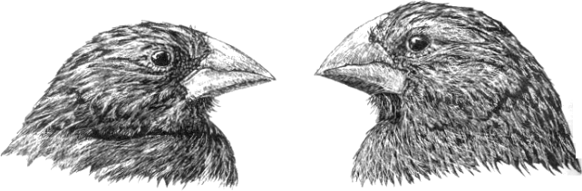
Peter, Rosemary Grant and co-workers performed a classic study on natural selection and evolution in wild populations by studying Darwin’s finches in the Galápagos archipelago. Almost all of the medium ground finches Geospiza fortis on the islet of Daphne Major were marked and measured over many years. The Galápagos islands are subject to extreme weather fluctuations, resulting in extremely wet (El Niño) and extremely dry (La Niña) weather conditions. The Grants analysed quantitative responses of birds to these extreme weather events, which cause population crashes and population booms respectively. In a way, the extreme conditions bring about ‘natural experiments’ by which scientists can study microevolutionary change in action. The Grants’ observations on patterns of morphological change were backed up with evidence of mechanisms responsible for change – they measured forces necessary to crack seeds of a particular size, and related these forces to selection on bill morphology. Their study shows the value of long-term studies under natural conditions in understanding evolutionary principles.

The famous evolutionary biologist J.B.S. Haldane once said 'No scientific theory is worth anything unless it enables us to predict something which is actually going on. Until that is done, theories are a mere game of words, and not such a good game as poetry’. The Grants’ study allows us to understand why selection brings about morphological change in populations, and because we understand the mechanisms that bring about the change, allows us to predict what changes may happen in future climatic events.

The data file that you have been given (Darwinsfinches.csv – available on Blackboard) contains a subset of data from the Darwin’s finch study. Data on bill depths are provided from Daphne birds before and after a La Niña -induced population crash, and birds from Santa Cruz 10 km distant. The aim of this practical is to use the data set to illustrate the four postulates of evolution by natural selection.

In statistical tests cite the test used, parameter values tested (e.g. means), a measure of variability (e.g. SDs), the test statistic and the degrees of freedom.

You have been provided with a comma separated values (csv) file – darwinsfinches.csv containing the following columns

Setting up analysis

You need to read in the data and refactor it slightly so all analyses will run smoothly

You need to set your working directory to where the data files are.

setwd("/PATH/TO/DATAFILES/”)

Alternatively, use the ‘Session’ command as follows:

1. Create a sub-directory named “R” in your “Documents” folder, and place the csv data file in it.

2. From RStudio, use the menu to change your working directory under Session > Set Working Directory > Choose Directory.

3. Choose the directory you’ve just created in step 1

Now read in the data

data <- read.table('darwinsfinches.csv', header = TRUE, sep = ',')

head(data)

str(data)

Finally, we need to make the survive and location columns a factor, because R currently thinks they are numeric.

data$survive <- factor(data$survive , levels=0:1, labels=c("Dead", "Alive"))

data$location <- factor(data$location , levels=0:1, labels=c("Daphne", "Santa"))

str(data)

You’re ready to go!

Postulate 1. Individuals within species are variable.

Produce histograms that classify the bill depths (Daphne Island (non-survivors and survivors done separately) and Santa Cruz island) into classes that show relatively fine resolution. Calculate means and SDs for each of the 3 distributions and present these in a Table.

Box 1.

Descriptive statistics, and producing Histograms in R

Descriptive statistics. To calculate the means and standard deviations for alive and dead birds on Daphne Major and all birds on Santa Cruz you can use a function called “tapply”, which does a similar thing to ‘function aggregate’ that you may already have met.  The syntax is as follows

tapply(dependent_variable, grouping_variable, function, na.rm)

The dependent variable is what we measure (bill depth). The grouping variable is how we separate our data (either survive or location). The function is what we want to do to the data. Finally na.rm will any rows featuring “NA” from the analysis if set to TRUE (we will always be setting it to TRUE).

Thus, if we want to calculate the mean, and standard deviation, bill depth for alive and dead birds on Daphne Major, we would use the following.

tapply(data$daphne_all, data$survive, sd, na.rm = TRUE)

Similarly, for the birds on Santa Cruz and Daphne Major

tapply(data$both_islands, data$location, mean, na.rm = TRUE)

tapply(data$both_islands, data$location, sd, na.rm = TRUE)

Histograms. Plot three histograms to show the distribution of bill depths of alive birds on Daphne Major, dead birds on Daphne Major, and birds on Santa Cruz. These correspond to the three columns in your data which you can derive using the table above.

To make your histograms comparable, you need to standardise the x-axes. To calculate your minimum and maximum x-values, you can use the functions max() and min() on the “both_islands” column of the table.

min_x <- min(data$both_islands - 2)

max_x <- max(data$both_islands + 1)

You can tell R to plot all three histograms in one figure with the following, which will plot the histograms on top of each other,

par(mfrow = c(3,1))

hist(data$alive, xlim = c(min_x, max_x), xlab = "", main = "