Hello, dear friend, you can consult us at any time if you have any questions, add WeChat: daixieit

Project 4

Parallel Programming with Machine Learning

Download the dataset from BB. Unzip  dataset.zip to folder  project4 .

The structure of working directory should look like below:

Task1: Train MNIST with softmax regression

Softmax regression (or multinomial logistic regression) is an extension of logistic regression that can handle multiclass classification problems. Softmax Regression, also known as Multinomial Logistic Regression, is an extension of Logistic Regression to the multi-class problem. The mathematical expression is as follows:

Suppose we have an input vector x ∈ Rn, and we want to classify it into one of K different classes.

For each class j, we have a weight vector wj ∈ Rn and a bias term bj.

We can compute the unnormalized log probabilities oj for x belonging to class j as follows:

zj = xT θj + bj

This gives us an output vector θ ∈ RK, where each element oj represents the unnormalized log probability of x belonging to class j.

We can then convert these unnormalized log probabilities into probabilities using the softmax function. The softmax function is defined as follows:

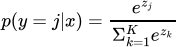
This gives us a probability vector p ∈ RK, where each element pj represents the

probability of x belonging to class j. This is the mathematical expression of softmax   regression. It maps an input vector x to a probability vector p, where each element pj represents the probability of x belonging to class j.

This process is also known as softmax classification. In practice, we usually choose the class with the highest probability as the predicted class.

For a multi-class output that can take on values y ∈ {1, … , k}, the softmax loss takes    as input a vector of logits z ∈ Rk, the true classy ∈ {1, … , k} returns a loss defined by:

Softmax gradient descent optimization algorithm : we need to compute the

gradients of the loss function with respect to the weights and biases, and then update the weights and biases. We can also write this in the more compact notation we

discussed in class. Namely, if we let X ∈ Rm×n denote a design matrix of some m

inputs (either the entire dataset or a minibatch), y ∈ {1, … , k}m a corresponding vector

of labels, and overloading ℓsoftmax to refer to the average softmax loss, then

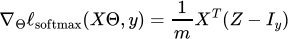
where

Z = normalize(exp(XΘ))  (normalization applied row-wise)

denotes the matrix of logits, and Iy  ∈ Rm×k  represents a concatenation of one-hot bases for the labels in y.

Here is the given training code in Python:

Note that for "real" implementation of softmax loss you would want to scale the logits to prevent numerical overflow, but we won't worry about that here (the rest of the

assignment will work fine even if you don't worry about this).

There are some functions inside the softmax function that you also need to fill in the details:

Function Declaration                                                                                What does the function do

matrix_dot(A, B, C, m, n, k)                                                                      perform a matrix multiplication operation between matrices A and B, and the result is stored in matrix C

matrix_softmax_normalize(A, m, n)                                                            apply the softmax activation function to the matrix A

vector_to_one_hot_matrix(y, Y, m, n)                                                         convert a vector y into a one-hot encoded matrix Y with dimensions m × n

matrix_minus(A, B, m, n)                                                                          perform element-wise subtraction between matrices A and B, with the result stored in matrix A

matrix_dot_trans(A, B, C, n, m, k)                                                              perform a matrix multiplication between the transpose of A and B, with the result stored in matrix C

matrix_div_scalar(A, scalar, m, n)                                                               divides all elements of matrix A by the scalar value scalar

matrix_mul_scalar(A, scalar, m, n)                                                              multiply all elements of matrix A by the scalar value scalar

matrix_minus(A, B, m, n)                                                                           subtracts matrix A from matrix B element-wise, , with the result stored in matrix A

softmax_regression_epoch_cpp(X, y, theta, m, n, k, lr, batch)                         train theta of softmax regression for 1 epoch

train_softmax(train_data, test_data, num_classes, epochs, lr, batch)               train a softmax classifier

a(l) = f(W(l)a(l−1) + b(l))

This process starts from the input layer, through the calculation of each layer’s weights and biases, as well as the activation function, and finally obtains the    predicted value of the output layer.

2. Backward Propagation (Training)

The training process of a neural network mainly updates the weights and biases  through the backpropagation algorithm. First, we need to define a loss function L to measure the gap between the predicted value and the true value. Then, we

update the weights and biases by calculating the gradient of the loss function for the weights and biases:

Here, ∂ ∂ a L

Here, α is the learning rate, which controls the step size of the update.

In this project, we are going to implement a 2-layer NN with SGD.

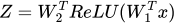
where W1 ∈ Rn×d and W2 ∈ Rd×k represent the weights of the network (which has a d- dimensional hidden unit), and where z ∈ Rk represents the logits output by the

network. We again use the softmax / cross-entropy loss, meaning that we want to solve the optimization problem.

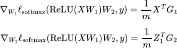
Using the chain rule, we can derive the backpropagation updates for this network (we'll briefly cover these in class, on 9/8, but also provide the final form here for ease of implementation). Specifically, let

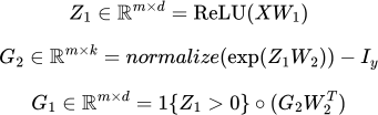
where 1{Z1 > 0} is a binary matrix with entries equal to zero or one depending on whether each term in Z1 is strictly positive and where ∘ denotes elementwise multiplication. Then the gradients of the objective are given by:

Here is the given training code in Python:

There are some new functions inside the NN function that you also need to fill in the details:

Function Declaration	What does the function do
matrix_trans_dot(A, B, C, m, n, k)	perform a matrix multiplication between   A and the transpose of B, with the result stored in matrix C
matrix_mul(A, B, size)	multiply matrix A from matrix B element- wise, with the result stored in matrix A
nn_epoch_cpp(X, y, W1, W2, m, n, l, k, lr, batch)	train the 2-layer NN for 1 epoch
train_nn(train_data, test_data, num_classes, hidden_dim, epochs, lr, batch)	train a 2-layer NN classifier

The outcome is like below:

The Extra Credit Policy

According to the professor, the extra credits in this project cannot be added to other projects to make them full marks. The credits are the honor you received from the professor and the teaching staff, and the professor may help raise you to a higher grade level if you are at the boundary of two grade levels and he thinks you deserve a better grade with your extra credits. For example, if you are among the top students    with B+ grade, and get enough extra credits, the professor may raise you to A- grade. Furthermore, the professor will invite a few students with high extra credits to have dinner with him.

Grading Policy for Late Submission

1. late submission for less than 10 minutes after the DDL is tolerated for possible issues during submission.

2. 10 Points deduction for each day after the DDL (11 minutes late will be considered as one day, so be careful)

3. Zero points if you submitted your project late for more than two days

File Structure to Submit on BlackBoard

<Your StudentID>.pdf  # Report

<Your StudentID>.zip  # Codes

├──	sbatch.sh
├──	src
│	├── nn_classifier.cpp
│	├── nn_classifier_openacc.cpp
│	├── simple_ml_ext.cpp
│	├── simple_ml_ext.hpp
│	├── simple_ml_openacc.cpp
│	├── simple_ml_openacc.hpp
│	├── softmax_classifier.cpp
│	└── softmax_classifier_openacc.cpp
└	test.sh

5 directories, 20 files