MATLAB For Scientists – FINAL EXAM
Hello, dear friend, you can consult us at any time if you have any questions, add WeChat: daixieit
MATLAB For Scientists – FINAL EXAM
Instructions
Answer the questions below in a single script. Submit the script titled Final_ studentID_script.m, to Canvas, by 12:00pm EST on 12/14. Separate each question with double percent signs and rewrite the main question prompt in a block of comments as shown below. Then, use comments to designate question sub-parts. Ensure each question follows the guidelines below:
. The display answer to every question should begin with the question # and part. Ex: for Q1 part a, disp(“Question 1a: “ + …) (-0.5 pts each).
. When specified, the answer should be displayed in a grammatically correct complete sentence, including spaces where appropriate, and punctuation marks (-0.5 pts each).
. Suppress all intermediate outputs. Only the answers should be displayed (-0.5 pts each).
. No hard coding beyond the minimal necessary (-0.5 pts each).
Problems
Problem 1 (60 pt.)
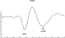
A visual evoked potential (VEP) measures the electrical signal of the visual cortex (a region of your brain) generated in response to a given visual stimulation. Examples of stimuli include flashes, alternating checkerboards, etc. In order to derive a reliable VEP response, a patient must be presented with multiple trials of the same stimulus. The VEP response is obtained by averaging the individual response of each trial. The figure on the right displays the results of a VEP response obtained by averaging 1000 trials collected in a healthy adult individual.
I. Load the signal an1.dat (you can use the function load). This variable contains 273 trials, and each trial is of length 107 samples. The signal is sampled at 350 Hz.
II. As described, the VEP response is obtained by averaging the individual trials point-by-point. The
obtained VEP should be a 1x10⁷ (or 107x1) vector and should resemble the figure above. Plot the VEP. The x-axis must be expressed in Time [ms] and the unit for the y-axis is Amplitude [µV]. Make sure that axes are labelled, the figure has a title, the thickness of the line plot is adequate for interpretation, etc.
III. After taking a more careful look at the data, the person in charge of analyzing the data noticed that
trials stored in the signal an1.dat include a period of time preceding the stimulus presentation. In fact, the stimulus was presented 250 ms after the recording of each trial was started. In other words, the
time vector should be redefined to account for the fact that the time = 0 ms (corresponding to the actual response) occurs 250 ms after the start of each trial. Plot the VEP and the newly defined time vector. Plot a vertical red line to indicate the new start time t = 0 ms. The time occurring before 0 should be indicated using negative values. The x-axis must be expressed in Time from stimulus presentation [ms] and the unit for the y-axis is Amplitude [µV]. Make sure that axes are labelled, the figure has a title, the thickness of the line plot is adequate for interpretation, etc. From now on, all the times are expressed with respect to the stimulus presentation.
IV. Compute the VEP response when including 75, 150, 225, and all trials. Plot them all in the same graph. The x-axis must be expressed in Time from stimulus presentation [ms] and the unit for the y-axis is Amplitude [µV]. Make sure that axes are labelled, the figure has a title, the thickness of the line plot is adequate for interpretation, etc. From now on, all the times are expressed with respect to the stimulus presentation.
V. N75 is defined as the amplitude of the negative peak of the VEP occurring between 65 and 75 ms. P100 is defined as the amplitude of the positive peak of the VEP occurring between 95 and 100 ms. Identify the values of N75 and P100. Display the answers in a grammatically correct complete sentence.
VI. A hot topic in the field of VEP research is the determination of the minimum number of trials needed to achieve reliable estimates of either N75 or P100. Compute the estimates of N75 and P100 by progressively increasing the number of trials averaged. In other words, considering N75, compute the first estimate by only considering 1 trial, the second by considering 2 trials, and the n-th by considering n trials, where the max of n is the maximum number of trials collected. Please do so for both N75 and P100. In the same graph, plot the series of N75 and P100 estimates as a function of number of trials included. Make sure that axes are labelled, the figure has a title, the thickness of the line plot is adequate for interpretation, etc.
Problem 2 (60 pt.)
During class we have been working on identifying cells and other biological structures, so I thought about pivoting to something more fun (M&M'S) for the final exam!
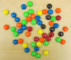
I. Load the image mms.jpg. Plot the image mms.jpg. The result should resemble the image on the right.
II. Subplot (1 row 3 columns) the R, G, and B layers of the original image.
III. By using the functions described in L8 and L9, design an algorithm for
the automatic detection of the number of M&M'S in the picture, please do so regardless of the color of the candies. Describe the approach utilized in your code (max 50 words). Display the answers in a grammatically correct complete sentence.
IV. Overlay and plot the boundaries of each candy to the original image.
V. By using the functions described in L8 and L9, design an algorithm for the automatic detection of the number of M&M'S in the picture, please do separately for each color. Describe the approach utilized in your code (max 50 words). Display the answers in a grammatically correct complete sentence.
VI. Bonus points: Overlay and plot the boundaries of each candy to the original image. The boundaries should be colored according to the actual color of each candy. In other words, the borders drawn around yellow candies should be yellow, etc.
2023-12-06