Hello, dear friend, you can consult us at any time if you have any questions, add WeChat: daixieit

ECON 460: Economic Applications of Machine Learrning

Fall 2021

Problem Set 2

        We will use the online spending application from the lecture notes lec04--fundamental.nb.html. First, create the variable yspend (10,000 observations with spending for each household) and the sparse matrix xweb, following the lecture notes (you can just copy the code from the lecture notes, and you don’t need to include this data preparation step when turning in the problem set).

1.) Recall that lasso selects a sparse model by zeroing out covariates. We will run a bootstrap experiment to see whether this model selection procedure is stable across different samples. In general, one should be cautious when applying bootstrap with the lasso (bootstrap CIs can fail to cover the true parameter with high probability), but we’re just using it to get a sense of the stability of lasso model selection.

a.) Run a lasso regression of log(yspend) on xweb, using 5-fold cross-validation to pick . Report the indices of the nonzero coefficients (you don’t have to report their names).

b.) Redraw a single “bootstrap” sample (same sample size as the original sample) by sampling from yspend and xweb with replacement. Run the lasso regression from part (a) on this bootstrap sample.

i.) Report the indices of the nonzero coefficients.

ii.) Report the indices of the coefficients that are nonzero only for the bootstrap sample.

iii.) Report the indices of the coefficients that are nonzero only for the original sample.

iv.) Report the indices of the coefficients that are nonzero for both samples.

c.) Based on these results, does the set of nonzero coefficients selected by the lasso seem to be stable across random draws of the data?

2.) We will run an out-of-sample experiment to see how well cross-validated lasso performs. First, draw a random sample of size n = 8, 000 from the original 10, 000 observations, without replacement. We will refer to these observations and as the “estimation” sample. We will refer to the remaining m = 2,000 observations  and as the “holdout” sample.

a.) Run 5-fold cross-validated lasso of log(yspend) on xweb on the estimation sample of n = 8,000 observations. Report a plot of the out-of-sample cross validation error as a function of (you can use the plot command on the cv.gamlr object as in the lecture notes).

b.) Let denote the optimal from part (a). Using the output of the lasso model with , compute the predicted value of log(yspend) at each in the holdout sample. Compute the in-sample prediction error of the cross-validated lasso:

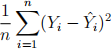
where denotes log(yspend) for observation i.

c.) Now compute the out-of-sample prediction error, using the holdout sample. Using the output of the lasso model with computed using the estimation sample i = 1, . . . , n, compute the predicted value of log(yspend) at each in the holdout sample. Call these predicted values . Compute the out-of-sample prediction error of the cross-validated lasso model on the holdout sample:

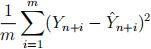
where denotes log(yspend) for observation n + i. How does this compare to the results from part (b)?