Hello, dear friend, you can consult us at any time if you have any questions, add WeChat: daixieit

EMAT10007 Introduction to Computer Programming

Coursework 2023

Overview

In this assignment, you will complete two computational modeling exercises.

Select one exercise from Part  1  (either  Exercise  1  or Exercise 2) and one exercise from Part 2 (either Exercise 3 or Exercise 4).

You are free to choose which exercise to complete for Part 1 and Part 2, but you must answer all of the questions for that exercise.

Each exercise will require you to take a real-life problem and translate it into a computer model in order to output a solution.

Use of packages

You are permitted to use the following Python packages for this coursework:

. matplotlib

. random

. math

.  csv

The use of any other packages will automatically result in a mark of zero for this coursework.

What you need to submit

Please submit a zipped (.zip) folder containing your work for each part (part1.zip, part2.zip):

1. All of the files that are needed to run your programme.  These include the Python (.py) file and any plain text data files. Your programme must be written as a .py file.

2. A README.txt plain text file that explains how your program should be run, for example which .py file should be run if there are more than one

3. A documentation.pdf file containing a report about your program (page limit:  1 page for Part 1, 1 page for Part 2, minimum font size: 11) Your report should explain how you wrote your program to answer each question of each exercise (e.g.  In Exercise  1,  Question  2 I used....).

. What programming techniques did you use and how did you use them to answer the question?

. Where and how did you reduce repetition in your code?

.  How did you make your code more modular (i.e.  making blocks of code easily re-usable)?

Part 1

Complete either Exercise 1 or Exercise 2

Exercise 1 - Measuring vegetation health

The NDVI, (Normalised Difference Vegetation Index), is a measure of the vegetation cover of a particular area. It is widely used in agriculture, forestry, and environmental studies to monitor the health and growth of plants.

Satellite or aerial remote sensing technology measures the reflection of light in the near-infrared (NIR) and visible red bands of the electromagnetic spectrum.

The NDVI, value in the range -1 to 1 is then calculated using the ratio:

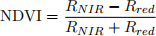(1)

where RNIR  is reflected NIR light and Rred  is reflected visible red light.

Figure  1:  Examples of typical percentage NIR and visible red light reflected from healthy and unhealthy vegetation

Table 1: Vegetation health associated with different categories of NDVI value

The file named part1_exercise1.zip on Blackboard contains data aerial data from the area of Cold Springs, Colorado, USA, which was affected by a wildfire in 2016. The data is taken from

Figure 2:  Aerial photograph of the Cold Springs area showing the four types of reflected light measured

a 2D aerial image recorded in 2019 as part of the National Agriculture Imagery Program (NAIP). It is divided into four .csv files that contain measurements of red, blue, green and NIR light in the image. Each .csv file contains a 4377 by 2312 array, where each pixel of the image is represented by an array element containing a number in the range (0, 255), representing the amount of reflected light in the pixel.

1. Your program should calculate the NDVI for each element in the 4377 by 2312 array, to 3 d.p.  using Equation 1.  It should then display the first 5 columns of the first 5 rows (5 by 5 array) of the full 4377 by 2312 array computed.

2. Your program should display the number of array elements in each category shown in Table 1.

3.  SWP (Stem Water Potential) is a sensitive indicator of water stress recorded directly from plant leaves.  SWP provides accurate information compared with indirect methods such as aerial imagery, but is labour intensive and time consuming.  NDVI values can predicted from SWP measurements using the equation:

NDVIp = 0.26 × SWP + 0.96                                              (2)

where NDVIp  is the predicted value.  Therefore, predicted NDVIp  values calculated using a small sample of SWP values (Equation 2), measured at different locations can be compared with aerially measured NDVI values (Equation 1) at these locations, to assess the accuracy of the aerially measured NDVI values.

A monitoring organisation recorded the SWP at different locations in Cold Springs over 4 years (Table 2). Your program should calculate and display the predicted NDVIp  values, to 3 d.p. for the year 2019, using the SWP values in Table 2 and Equation 2.

Table 2: SWP recorded at five locations in Cold Springs [Column 1 updated 27 November 2023]

4. Your program should compute the root mean square error (RMSE) between the predicted NDVIp  values  (computed in Question 3) and NDVI values found in Question  1), for 2019. The (x, y) location shown in Table 2 is the same as the (x, y) index of the corresponding element within the 4377 by 2312 aerial data array.

For this question, the RMSE can be defined as

(3)

where y is a predicted data series, ˆ(y) is a measured data series, and N is the number of data points. Your program should display the RMSE to 3 d.p.

5. Your program should output a line plot showing the NDVIp   (vertical axis) for each year (horizontal axis), using the information in Table 2.  The data for each location should be displayed as a separate line on the plot, shown on the same axis.   Finally,  your program should save the plot as a file with the name ex1_question5.png.

Exercise 2 - Microbes

Computational models of how microbial communities grow in various environments is used for explaining experimental results, and making predictions about the dynamics of microbial commu- nities that can be tested experimentally.

In this exercise you will create a 2-dimensional model to simulate the behaviour of a microbial community within a 200 unit by 200 unit observation chamber.

The chamber also contains a food source at location (fx, fy) = (50, 150), and a constant force due to fluid flow, F, which acts in the negative y direction.

Figure 3: Observation chamber showing the microbes, the food source and the constant force, F.

1.  Create 300 data points on a scatter plot, where each data point represents a single microbe. Assign each microbe, m, a randomly generated initial position (mx, my), where mx  and my are integers and are within the chamber (i.e. the initial position must not lie on the boundary, or outside, of the chamber). Assume that more than one microbe may occupy the same initial position.

Assign each microbe a randomly generated integer value in the range 1 to 14 to represent its size.  The markers on the scatter plot can be of uniform size and do not need to reflect the size of the individual microbes.

2. Your program should update the position of each microbe at each timestep, for 100 timesteps. The position a microbe at time t is determined by Equation 4 and Equation 5.

Horizontal position:

mx,t = mx,t− 1 + Mrx+ Mcx                                                                    (4)

Vertical position:

my,t = my,t− 1 + Mry + Mcy + MFy                                                            (5)

where:

.  Mrx  and Mry  are each a randomly generated integer in the range -5 to 5, representing random motion of the microbe in the horizontal and vertical direction respectively.

.  Mcx and Mcy represent horizontal and vertical motion due to chemotaxis (motion towards a chemical attractant such as a food source):

Mcy  = e(fy − my,t− 1 ) (5)

Mcy  = e(fy − my,t− 1 ) (5)

where the strength of attraction, e, is found by calculating r using Equation 8, (where mx = mx,t− 1 , my  = my,t− 1 ), and then using lookup table, Table 3.

(8)

Table 3: Strength of attraction, e, for different values of r

.  Mfy represents the movement due to fluid flow, and has a constant value, Mfy  = −0.025

If the new position (mx,t− 1 , my,t− 1 ) is not within the observation chamber boundary, the mi- crobe should remain at its previous position position (mx,t,my,t) and not move to the new position.

Every 20 timesteps, your program should save the plot as a .pdf file with the title:

.  ex2_question2_plot0.pdf (timestep = 0)

.  ex2_question2_plot1.pdf (timestep = 1)

.  ex2_question2_plot2.pdf (timestep = 2)

.  ex2_question2_plot3.pdf (timestep = 3)

.  ex2_question2_plot4.pdf (timestep = 4)

.  ex2_question2_plot5.pdf (timestep = 5)

The plot saved should show only the position of microbes in the current timestep, and the axes should have the range 0 to 200 in all figures.

3. After updating the microbe position and before plotting the microbe, your program should also update the size of each microbe at each timestep.  The size, s of a microbe at time t is determined by Equation 9:

(9)

where:

. r is calculated using Equation 8, (where mx = mx,t , my  = my,t)

.  Mx , My  are the distance moved by the microbe in the horizontal and vertical direction between time t − 1 and time t  (remember the distance moved is zero if the the new position generated (mx,t− 1 , my,t− 1 ) was not within the observation chamber boundary.

4.  Microbe death: Your program should remove any microbes with size, st, less than or equal to 0 from the simulation, so that they are not plotted from the current timestep onwards.

Microbe reproduction: Your program should replace any microbes with size st  greater than or equal to 20 with two microbes at the same location as the original microbe, but with size st/2 before plotting.

5.  Generate some statistics about the colony. At 100 timesteps:

(a) How many living microbes are in the colony?

(b) What is the average concentration (microbes per unit area) within a radius of 25 units from the food source?

Part 2

Complete either Exercise 3 or Exercise 4

Exercise 3 - Running on renewables

In this exercise you will explore the pros and cons of using solar and wind power.  The file named part2_exercise3.zip on Blackboard contains data of the solar intensity I and wind speed v at an address in the UK. The data is divided into months.   The  data for each month consists of measurements taken throughout an average day in one-hour intervals starting at 12 am (0000 hrs) and ending at 11 pm (2300 hrs).  The solar intensity data is in units of W/m2 .  The wind speeds have units of miles per hour.

The power describes the rate of energy production and consumption.  The power produced by a solar panel is given by the equation

Psolar = εWHI                                                             (10)

where ε is the efficiency of the solar panel, W and H are the width and height of the solar panel, and I is the solar intensity.  Since I varies with time, the solar power Psolar  will also vary with time. In this problem you will consider three types of solar panels; their parameter values can be found in Table 4.

Table 4: Parameter values for three types of solar panel.

1. Using the solar intensity data for December and Equation (10), compute the power every hour starting from 12 am and ending at 11 pm for each type of solar panel.  Plot the results (power versus time) on the same figure. Save this figure as a file called ex3_question1.pdf. Print the maximum power of produced by each type of solar panel to the screen along with a message stating which type of solar cells produced the greatest power.

2.  Suppose that a house needs 250 W of power in order for the heating to work.  The house has 10 solar panels of type A. Determine the percentage of hours in December when the total power is less than 250 W and print a message with this value to the screen.   This is the percentage of hours when the house needs an alternative power source to provide energy for heating. The power of 10 panels is 10 times the power of a single panel.

3.  Using solar panel type A, compute the average power that is produced during a single day for each month. That is, for each month, compute the power at each time from 12 am to 11 pm and then average the results. Do this for each month.  Create a plot that shows the average power versus month.  Save this figure as a file called ex3_question3.pdf.  You should see that the summer months lead to more power being produced on average.

The power produced by a wind turbine is given by the equation

(11)

where K and f are efficiency factors and ω is the rotation rate of the turbine.  The rotation rate is measured in rad/s.  The rotation rate of a wind turbine changes in time and is affected by the wind speed v.  If vn  and ωn  represent the wind speed and the rotation rate at time tn   (e.g.  12:00 am), then the rotation rate one hour later (e.g. 1:00 am) can be obtained from the formula

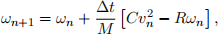(12)

where ∆t = 3600 s, and M , C, and R are constants that relate to the geometry, aerodynamics, and friction of the turbine.  The wind speeds in the data have units of miles per hour.  This will need to be converted into meters per second (1 mile per hour = 0.44704 meters per second).  The parameter values for the wind turbine can be found in Table 5.

Table 5: Parameter values for the wind turbine.

4. Using the wind-speed data along with Equations (11) and (12), calculate the power produced by wind turbine at one hour intervals starting from 12 am and ending at 11 pm in July. You can assume that the wind turbine is initially motionless, ω0  = 0 rad/s.  Create a plot of the rotation rate as a function of time.  Save this figure as a file called ex3_question4.pdf. Print the value of the wind power at 5 pm.

5. Assume that a house has 6 solar panels of Type A and one wind turbine.  Compute the total power, Ptotal  = 6Psolar  + Pwind, at one hour intervals starting from  12 am on 1st June and ending at 11 pm on 31st December.  You may assume that the solar intensity and the wind speed is the same for each day in a month, and that the turbine is initially motionless ω0  = 0 rad/s. Then use the series you have generated for 12 am on 1st June and ending at 11 pm on 31st December to create a plot that shows the total solar power, the wind power, and total power at one hour intervals starting from 12 am and ending at 11 pm on 1st December. Save this figure as a file called ex3_question5.pdf. You should see that the wind turbine produces a steady power throughout the day, while the solar power only spikes around mid-day. Print a message that states whether the total power ever drops below 250 W in December.