Math 9 2023 Fall Final Project Description
Hello, dear friend, you can consult us at any time if you have any questions, add WeChat: daixieit
Math 9 2023 Fall Final Project Description (Section A & B)
Numerical solutions and Applications of the SIR model
This final project serves as the open note programming final exam of this course, counting 20 points (20%) in the total grades. The “step size” in grading is 0.5 points, meaning that whenever one requirement below is not satisfied, at least 0.5 points will be subtracted.
Due Date: 11:59 pm December 10th, Sunday. NO EXTENSION. Graded as 0% automatically for any submission after this deadline.
Submission: upload the report in the format of MATLAB live script file to Canvas. The submission should be a well-organized and well-written report, which means:
(1) All sections are well-structured, with appropriate section titles.
(2) All figures are clear and have necessary figure captions (or descriptions) as text. (3) Have necessary descriptions/answers for the required parts/questions.
(4) Have basic comments for your MATLAB codes providing an overview of each code block.
(5) All code blocks should already be executed, have the required outputs, and suppress the unnecessary outputs.
(6) All formulas should be presented in the text blocks using the “Insert - Equation” function. (7) All functions should be in-script functions (defined at the end of the live script file).
Please include everything in one single live script file (.mlx file) , any other formats (.pdf, .doc, .m file, Jupyter notebook, …) or redundant files are not valid and will be graded as 0% automatically.
Submitting merely the codes and/or incomplete results will severely impact your grades.
Your report should address all the tasks listed in this file.
Task 1 (1pt)
1. (At the beginning of your report) Give your report an appropriate title reflecting its scientific
contents (don’t simply name it as “Math9 Final Project”).
2. Write your student id and name under the title.
3. Rename your live script file to "Math9_FinalProject_your name_yourID.mlx".
4. Acknowledgeing the final project policy by reading and copying the following paragraph (displayed in Italic font) at the beginning of your report (as a separate section) and keeping the requirements in mind.
I hereby confirm that the present report is my own work. If any texts or codes from books, papers, the Web, or any other sources have been copied or in any other way used, all references have been acknowledged and cited. Iam aware that the instructor has the authority to report and investigate any potential academic misconduct in this course, and such misconduct could lead to failing this course. If I have employed any AI models (including but not limited to ChatGPT), I have appropriately and explicitly acknowledged their use in the report whenever the results were generated with the aid ofAI.
Task 2 (4pt)
1. Search and read online resources and articulate, then use your own words to briefly discuss what a mathematical model is, and its significance in the study of infectious diseases (100~300 words).
2. Read the assigned part of the following online materials, which should provide you a
comprehensive introduction of the SIR model:
2.1. Compartmental models in epidemiology – read the SIR model part.
2.2. SIR Modeling – read the first four sections.
3. Assume the total population N is a constant, and divide N into three groups: susceptibles, infectives, and recovered/removed. Then we denote:
S(t) = proportion of susceptiblesattimet;
I(t) = proportion of infectivesattimet;
R(t) = proportion of recovered/removed at time t.
Write the following standard SIR model on your live script file using “Insert -- Equation” function:
![]() = −βIS,
= −βIS,
![]() - = βIS − YI
- = βIS − YI
![]() = YI.
= YI.
And explain the biological meaning of all the terms, variables and parameters. 4. Answer the following questions:
4.1. What is the biological meaning of the term βIS ? Why does it have the negative sign?
4.2. Why does the right-hand side of the third equation only have one term? What does it mean?
4.3. One of the major assumptions of this standard SIR model is: S(t) + I(t) + R(t) = 1 is a constant. Practically speaking, under what circumstances can we make such an assumption?
4.4. The basic reproduction number is defined by R0 = ![]() , what is its biological meaning? And what will happen ifR0 > 1?
, what is its biological meaning? And what will happen ifR0 > 1?
4.5. Search for online materials and provide an example (from news/articles/research papers) that during the COVID- 19 pandemic, R0 > 1 held for a quite longtime.
Task 3 (7pt)
Consider the following situation: people in a small town (total population: 10000) are experiencing the flu season, and today's record shows that 10 people have already recovered, and 200 people are having the flu. Assume that active immunity is obtained once fully recovered, and the newborn and death can be neglected during a short period of time. Here we also assume that the rate of infection when contacting a patient is 75%, and every day a patient has a probability of 15% of becoming fully recovered (rate of recovery).
1. Based on the above information, write down the SIR model, clearly indicate the initial condition and parameter values.
2. Use ode45 (a MATLAB built-in toolbox, very similar to the ode23) to simulate the trend of these three groups within the next 45 days (time unit: day). When writing the function for this SIR mode, name it “simple_SIR”, and make sure the parameters ![]() and ’ are also part of the function inputs.
and ’ are also part of the function inputs.
3. Plot simulation results in one figure using the plot function.
4. Polish your plot, add a figure title, give appropriate names for both two axes, adjust the linewidth of the curves, and change the labels of the legend to "S", "I", "R".
5. Interpret your simulation result, briefly explain what may happen in the next 45 days.
6. What is the basic reproduction number in this case? What is the basic reproduction number if the infection rate is only 10%? What will your simulation be like?
7. Assume we can reduce the infection rate to 40% by keeping social distance , and increase the recovery rate to 25% by using stronger medication, what your simulation will be like? (You should have a new plot with appropriate title, axes labels, and legend, and provide necessary interpretation.)
Task 4 (2pt)
In the earlier scenario, we assumed that the infection and recovery rates were constant, which is not entirely realistic. For example, the rate of infection is influenced by various factors such as mask usage, proximity, the health condition of individuals, and more. Instead of introducing new variables to account for these uncertainties, we incorporate randomness into our model to capture these fluctuating elements. Here, we consider the infection rate as a random variable ranging from 30% to 90%, and the recovery rate as a random variable spanning from 10% to 30%. Both rates follow auniform distribution within theirrespective ranges.
1. Based on the above assumptions, write a new function for the improved SIR mode and name it “simple_SIR_2” . You should generate the random infection and recovery rates inside your “simple_SIR_2” function.
2. Use ode45 to simulate the trend of these three groups (S, I, and R) within the next 45 days (time unit: day).
3. Run your simulation 20 times and plot all results in the same figure. Color your curves of the three groups (S, I, andR) in blue, red, and yellow, respectively. (Your figure has an appropriate
title, axes labels, and legend.)
4. Interpret your simulation results.
Task 5 (4pt)
The Hong Kong flu, also known as the 1968 flu pandemic, was a flu pandemic whose outbreak in 1968 and 1969 killed between one and four million people globally. Read the online materials to learn more about the Hong Kong flu:
This flu pandemic also affected New York City (population: approximately 7,900,000 in the late 1960's), and the table below shows the weekly totals of "excess" pneumonia-influenza deaths, which can be understood as the deaths caused by the flu epidemic (Source: Centers for Disease Control):
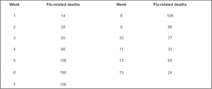
1. Input the above data into MATLAB (your live script) and visualize the data using bar plot. In
your figure, the labels of x andy axes should be “Week” and “Excess deaths”, respectively.
2. Since this data can be understood as the deaths caused by the flu epidemic, based on the death rate of the Hong Kong flu, we assume that the above numbers are approximately 1/500 to the weekly total infectives population. Based on this assumption, scale the data, and visualize it using scatter plot. The labels of x and y axes should be “Week” and “Estimated infectives”, respectively.
3. Use the standard SIR model (“simple_SIR”) and ode45 to simulate the trend of these three groups (S, I, and R) from day 0 to day 100 (time unit: day). The initial conditions: total population = 7,900,000, total suspectibles = 7,900,000- 14*500, total infectives = 14*500, total recovered/removed = 0. Infection rate = 0.5,recovery rate = 0.6. Plot your simulation result.
4. Plot your “Estimated infectives” data and your simulation result of the infectives group in one figure and compare the difference. (When plotting the “Estimated infectives” data, the first point should be at day 0, the second point is at day 7, …, and the last point is at day 84.) Calculate the absolute error between your simulation and the “Estimated infectives” data at each corresponding time point and summarize all the errors (and name it "fitting_err").
5. Change the infection rate and see if you can find a value that can improve your simulation results (i.e., has a smaller fitting_err), show your plot.
Task 6 (1pt)
Use no lease than 100 words to briefly discuss what you have learned about the SIR model, and how the numerical simulations help you understand the model and the control of an infectious disease. And more importantly, raise at least three limitations of this model (i.e., how to improve the model to make it more practical). You do not need to write any MATLAB code in this section.
Task 7 (1pt)
1. The title should use “Title” font.
2. Format each task (from Task 2 to 6) into one section, separate by section break, and give an appropriate section title (using “Heading 1” font).
3. Add one more section titled “References”, and list all the materials (including AI models) that you used (you do not need to list the materials provided in Task 2).
4. Add one more section titled "Acknowledgement”, and list all the people (besides the instructor and TAs) that helped you on your final project.
5. Execute all your code and only show the required outputs.
Optional Task (Ungraded)
1. In Task 5, we experienced how to manually tune the parameter values to make our simulation abetter fit (i.e., a smaller fitting error) for the data. However, it is almost impossible for us to find the parameter values that can minimize the fitting error, especially when we have multiple parameters. Luckily, MATLAB has a built-in toolbox named fminsearch, that can help us minimize the fitting error. Learn how to use fminsearch and apply it to our Task 5 to find the parameter values of β andy that minimize the fitting error and plot the corresponding result.
2. Recall in Task 2, we mentioned that one of the major assumptions of the standard SIR model is that the total population is a constant, which is also called “SIR model without demography” . 2.1. Learn the “SIR model with demography” via online materials and develop the corresponding model with “birth rate = mortality/death rate = μ” and interpret the model (similar to Task 2).
2.2. Use ode45 to simulate the trend of these three groups (S, I, andR) from day 0 to day 100 (time unit: day). The initial conditions: total population = 7,900,000, total suspectibles = 7,900,000- 14*500, total infectives = 14*500,total recovered/removed = 0.
2.3. Use fminsearch to find the optimal parameter values that provide the best fit of the “Estimated infectives” (Task 5) and plot your result.
2023-12-04
Numerical solutions and Applications of the SIR model