MSiA 400 Lab Assignment 3
Hello, dear friend, you can consult us at any time if you have any questions, add WeChat: daixieit
MSiA 400 Lab Assignment 3
Due Dec 3rd at 11:59pm
Instructions: Please submit a report file that includes: a short answer, related code, printouts, etc. for each problem (where necessary). Push your answers to Github or Canvas. All programming must be in R (or R Markdown).
Problem 1
I rolled a 6-sided die 100 times and observed the following results:

Problem 1a
What is the maximum likelihood estimate for the dice roll probabilities θ = (θ1 , · · · , θ6 )?
Problem 1b
Assume the prior θ ∼ Diri(1). I.e., assume that prior over roll probabilities are uniform Dirichlet with prior α = 1 (the Dirichlet distribution is a multivariate generalization of the beta distribution, with probability distribution function 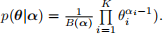 I.e., use a prior assumption that the die is fair and using six artificial rolls (one on each face) to incorporate this prior.
What is the posterior log-likelihood of the above rolls (in terms of θ)? What is the maximum a posteriori estimate for θ?
Problem 2
I have one fair die (all rolls have 1/6 probability) and one weighted die, with roll probabilities as follows:
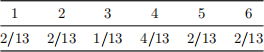
Model dice rolls as a Hidden Markov model, with the hidden state corresponding to whether or not the die is fair. Assume initially die is fair/unfair with 50/50 probability and there is a probability of 25% (after each roll) that I swap the dice. The following rolls are observed:
4, 4, 5, 2, 2, 6
Problem 2a
What is the likelihood of the observation and all the hidden states are dice being fair? What is the likelihood of the observation and all the hidden states are dice being not fair? Which is more likely?
Problem 2b
What is the most likely sequence of hidden states conditioning on the observations? (Hint: You may want to look up Viterbi algorithm for HMM)
Problem 3
You will further analyze the gradAdmit.csv dataset (from Lab 4 and Assignment 2). As a reminder, this dataset contains a list of students (rows), along with whether or not they were admitted to graduate school (admit), their GRE score (gre), their GPA (gpa), and the prestige of their undergraduate university (rank). You do not need to repeat the parameter tuning from Assignment 2.
Problem 3a
Compute the class balance for both the training set (80% from Assignment 2) and test set (20%). For each dataset, what percentage of students were admitted?
Problem 3b
Using your optimal parameters from Assignment 2, Problem 1c, and the model trained on the full training set (if you did this improperly before, redo it), compute the precision, recall, and specificity of the test dataset. Hint: the confusionMatrix function may be helpful.
Problem 3c
Based on your answer to Problem 3a, what percentage of minority over-sampling would create the most even class balance? Generate that many artificial training samples using the SMOTe algorithm (you may use the SMOTE function). Combine the original training dataset with the generated dataset and confirm the class balance is as desired.
Problem 3d
Retrain your model on the combined training dataset (using the same parameters). Compute the precision, recall, and specificity of the test dataset. Note: the test dataset should not be augmented. How do they differ from Problem 3b?
Problem 4
Use importance sampling and the Monte Carlo integration method to estimate the integral  sin xdx. 10π
Use 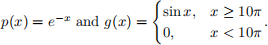 Note: this problem is similar to Assignment 1, Problem 2.
Problem 4a
What is the probability of drawing a sample x ≥ 10π from the exponential distribution (with λ = 1), i.e. p(x ≥ 10π)?
Problem 4b
What is the exact solution to the integral, i.e., the result obtained via calculus? You may use the result given in Assignment 1, Problem 2: 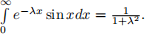
Problem 4c
Pick a biasing distribution that should work well for this problem. Your goal is to minimize the variance. Explain your choice. Note: choosing p*(x) > p(x) when g2(x)p(x) is large and p*(x) < p(x) when g2(x)p(x) is small reduces the variance.
Problem 4d
Numerically estimate the integral using the importance sampling method with the biasing distribution from Problem 4c and number of samples n = 106.
2023-11-28