Hello, dear friend, you can consult us at any time if you have any questions, add WeChat: daixieit

Assignment 3

COMP 250

Fall 2023

posted:            Friday, Nov.  17, 2023

due:                 Monday, Dec. 4, 2023 at 23:59

General Instructions

For this assignment need to download the files provided. Your task is to complete and submit the following file:

DecisionTree.java

• Do not change any of the starter code that is given to you.  Add code only where instructed, namely in the “ADD YOUR CODE HERE” block. You may add private helper methods to the class you have to submit, but you are not allowed to modify any other class.

• To run the code in Eclipse, you will need to use the default package and not have a package statement. (The reason for this constraint has to do with the use of serialization.  We have tried to make it run in other packages but we not able to at the time of the assignment release.  We will update you if we find a solution.)

•  You are NOT allowed to use any class other than those that have already been imported for you.

Any failure to comply with these rules will give you an automatic 0.

•  Do NOT start testing your code only after you are done writing the entire assignment.  It will be extremely hard to debug your program otherwise. If you need help debugging, feel free to reach out to the teaching staff.  When doing so, make sure to mention what is the bug you are trying to fix, what have you tried to do to fix it, and where have you isolated the error to be.

Submission instructions

•  Submissions will be accepted up to 2 days late. Remember that you each have 2 free late days to use this semester. Any additional late day will be penalized by 10 points per day. Note that submitting one minute late is the same as submitting 23 hours late. We will deduct points for any student who has to resubmit after the due date (i.e. late) irrespective of the reason, be it the wrong file submitted, the wrong file format submitted or any other reason. We will not accept any submission after the 2 days grace period.

•  Don’t worry if you realize that you made a mistake after you submitted: you can submit multiple times but only the latest submission will be evaluated. We encourage you to submit a first version a few days before the deadline (computer crashes do happen and Ed Lessons may be overloaded during rush hours).

1    Introduction

Congratulations!  You have just landed an internship at a startup software company.  This company is trying to use AI techniques – in particular decision trees – to analyze spatial data.  Your first task in this internship is to write a basic decision tree class in Java. This will demonstrate to your new employer that you understand what decision trees are and how they work.

From a quick web search, you learn that decision trees are a classical AI technique for classifying objects by their properties. One typically refers to object attributes rather than object properties, and one typically refers object labels to say how an object is classified.

As a concrete example, consider a computer vision system that analyzes surveillance video in a large store and it classifies people seen in the video as being either employees or customers.  An example attribute could be the location of the person in the store. Employees tend to spend their time in different places than customers. For example, only employees are supposed to be behind the cash register.

For classification problems in general, one defines object attributes with x variables and one defines the object label as a y variable. In the example that you will work within this assignment, the attributes will be the spatial position (x1 , x2 ), and the label y will be a color (red or green).

Let’s get back to decision trees themselves.  Decision trees are rooted trees.  So they have internal nodes and external nodes (leaves). To classify a data item (datum) using a decision tree, one starts at the root and follows a path to a leaf. Each internal node contains an attribute test. This test amounts to a question about the value of the attribute – for example, the location of a customer in a store.  Each child of an internal node in a decision tree represents an outcome of the attribute test.  For simplicity, you will only have to deal with binary decision trees, so the answers to attribute test questions will be either true or false. A test might bex1  < 5. The answer determines which child node to follow on the path to a leaf.

The labelling of the object occurs when the path reaches a leaf node. Each leaf node contains a label that is assigned to any test data object that arrives at that leaf node after traversing the tree from the root. The label might be red or green, which could be coded using an enum type, or simply 0 or 1. Note that, for any test data object, the label given is the label of the leaf node reached by that object, which depends on the outcomes of the attribute tests at the internal nodes.

This document should give you enough information about decision trees for you to do the assignment. If you wish to learn more about decision treees, then there are ample resources available on the web.  Steer towards resources that are about decision trees in computer science, in particular, in machine learning or data mining. For example:

https://en.wikipedia.org/wiki/Decision_tree_learning

Be aware that these resources will contain more information than you need to do this assignment, and so you would need to sift through it and figure out what is important and what can be ignored. Feel free to use Ed to share links to good resources and to resolve questions you might have. The task of understanding what decision trees are is part of the assignment. The amount of coding you need to do is relatively small, once you figure out what needs to be done.

Data:  A decision tree, and an unlabelled data item (datum) to be classified

Result: (Predicted) classification label

CLASSIFY(node,datum) {

if node is a leaf then

return the label of that node i.e. classify;

else

test the data item using question stored at that (internal) node, and determine which child node to go to, based on the answer ;

return CLASSIFY(child,datum);

end

}

2 Instantiating the decision tree problem

For this assignment, the problem is to classify points based on their position. Each datapoint has an array of attributes x, and a binary label y (0 or 1).  For this section, we will focus on datapoints with only two attributes.

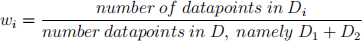
A graphical representation of example of a data set looks like this. (For the graphs, the attribute value x[0], is represented as x1 and x[1] as x2.) For those who print out the document in color, the red symbols can be label 0 and the green symbols can be label 1. For those printing in black and white, the (red) disks are label 0 and the (green) ×’s are label 1.

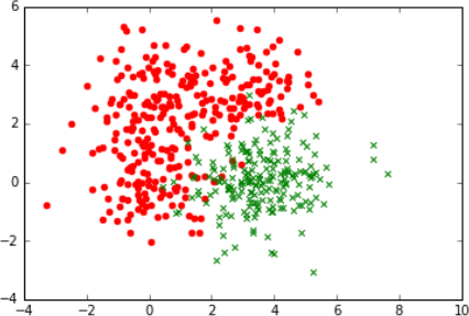
Figure 1: x1  is horizontal and x2  is vertical coordinate.  Note that the points are intermixed.  There is no way to draw a horizontal or vertical line or any curve for that matter that could split the data.

2.1 Finding a good split

Now that we have an idea of what the data are, let us return to the question of how to split the data into two sets when creating a node in a decision tree. What makes a ‘good’ split? Intuitively, a split is good when the labels in each set are as ‘pure’ as possible, that is, each subset is dominated as much as possible by a single label (and the dominant label differs between subsets). For example, suppose this is our data:

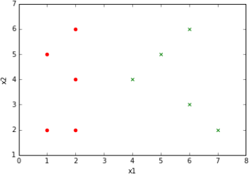
Figure 2: What would be a good split of this data?

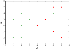
Two of many possible splits we could make are shown in Fig. 3. Fig 3-a splits the data into two sets based on the test condition (x1   < 4),i.e. true or false. (By definition, the green symbol that falls on this line is considered to be in the right half since the inequality is strict.) This is a good split in that all data points for which the test condition is false have the same label (green) and all data points for which the test condition is true have the same label (red), and the labels differ in the two subsets.

The split condition (x1  < 6) in Fig. 3-b is not as good, since the subset for which the condition is true contains datapoints of both labels.

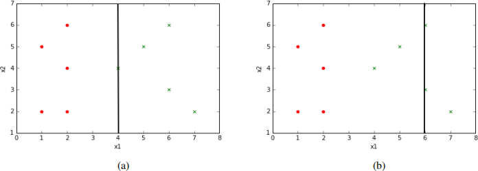
Figure 3: Example of different splits on the x1  attribute.

Splits can be done on either of the attributes.  For the example in Fig. 4-a, a good split would be defined by the test condition (x2  < 4).

The situation is more complicated when the data points cannot be separated by a threshold on x1  or x2 , as in Fig 4-b, however. It is unclear how to decide which of the three splits is best.  We need a quantitative way of deciding how to do this.

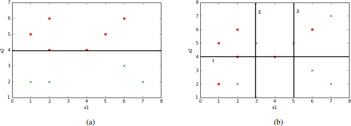
Figure 4: (a) Example of a data set and a split using the x2  attribute, where the two subsets have distinct labels. (b) An example of a data set in which there is no way to split using either an x1  or x2  value, such that the two subsets have distinct labels.

2.2 Entropy

To handle more complicated situation, ones needs a quantitative measure of the ‘goodness’ of a split, in terms of the impurity of the labels in a set of data points. There are many ways to do so. One of the most common is called entropy.1 The standard definition2 of entropy is:

where p(i) is a function such that 0 ≤ pi  ≤ 1 andΣipi  = 1. Note that the minus sign is needed to make H positive, since log2 pi  < 0 when 0 < pi < 1. Also, note that ifpi = 0 then pi log2 (pi ) = 0 since that is the limit of this expression as pi → 0. (Recall l’Hopital’s Rule in Calculus 1.)

For the special case that there are two values only, namely p1  and p2  = 1−p1 , entropy H is between 0 and 1, and we can write H as a function of the value p = p1. For a plot of this function H(p), see:

https://en.wikipedia.org/wiki/Binary_entropy_function

In this assignment, we use entropy to choose the best split for a data set, based on its labels.  We borrow the formula for entropy and apply it to our problem as follows:

where

• L isthe set of labels, andy is a particular label

• D is a data set; each data point has two attributes and a label i.e. (x1 , x2 , y)

• H(D) is the entropy of the dataset D

• p(y) is the fraction of data points with label y from dataset D.

Since L consists of only two labels, entropy is between 0 and 1. Entropy is 0 if p(y) takes values 0 and 1 for the two labels. Entropy is 1 if p(y) = 0.5 for both labels.  Otherwise it has a value strictly between 0 and 1. See plot in the link above.

2.3 Using entropy to define a good split

During the training phase, when one constructs the decision tree, a node is given a data set D as input. If D has entropy greater than 0, then we would like to split the data set into two subsets D1  and D2 . We would like the entropy of the subsets to be lower than the entropy of D.  The subsets may have different entropy, however, so we consider the average entropy of the subsets. Moreover, because one subset might be larger than the other, we would like to give more weight to the larger subset. So we define the average entropy like this:

H(D1 , D2 ) = w1 × H(D1 ) + w2 × H(D2 )

where wi is the fraction of the points in subset i,

and i is either 1 or 2. Note that w1  + w2  = 1.

NOTE: DO NOT use the formula : w2  = 1 - w1 , although correct, this leads to a numerical approximation error. For each of the weights (w1 , w2 ) use the formula mentioned above separately.

ASIDE: (We mention the following because you will likely encounter it in your reading.) When building a decision tree, one often considers the difference H(D) − H(D1 , D2 ), which is called the information gain. For example, one may decide whether or not to split a node based on whether the information gain is sufficiently large. In this assignment, you will instead use a different criterion to decide whether to split a node when building the decision tree Your criterion will be based on the number of data items in D, as will be discussed later.

2.4 Example

Let us now return to the examples we saw earlier and use entropy to discuss which split is best. Recall the example of Fig. 4-b. To calculate the entropy of the dataset D before split, note there are two classes with 6 points in each of the classes. So the fraction of points in each class is 0.5 and the entropy is:

•  Split 1 breaks the dataset into two sub datasets, where the subdataset on top contains 8 points (5 red dots , 3 green crosses) and the one below has 4 points (1 red dot, 3 green crosses). Calculating average entropy H(D1 , D2 ) after the split yields:

•  Split 2 breaks the dataset into two sub datasets, where the sub dataset on the left has 5 datapoints (4 red dots, 1 green cross) and the other one has 7 datapoints ( 2 red dots , 5 green crosses).  The average entropy H(D1 , D2 ) after the split is:

•  Split 3 breaks the dataset into 2 sub datasets, where the sub dataset on the left has 7 datapoints (5 red dots, 2 green crosses) and the other one has 5 datapoints ( 1 red dot , 4 green crosses). The average entropy H(D1 , D2 ) after the split is:

So, split 2 and 3 have lower average entropy than split 1.  It is no problem that split 2 and 3 have the same average entropy.  Either one can be chosen as the ‘best split’ .  For the assignment, select the first encountered best split when the check for the best split starts from the first attribute (x[0]) and proceeds from there and for a given attribute the check starts from the first datapoint and proceeds thereafter.

2.5 Finding the best split

We can use entropy to compare the ‘goodness’ of different splits.  The simplest way to define the best split is just to consider all possible splits and choose the one with the lowest average entropy.  In this assignment, you will take this brute force approach.  You will consider each attribute x1  and x2  and each of the values of that attribute for points in the data set. You will compute the average entropy for splitting on that attribute value, and you will choose the split that gives theminumum.

Figure 5: Example of an overfit decision tree on the outlier dataset