Hello, dear friend, you can consult us at any time if you have any questions, add WeChat: daixieit

ME 280, Fall 2021

Assignment 2

Consider the following boundary value problem (BVP): Given f(x), g and q, find u(x) such that

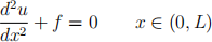
where .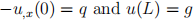

You are to write and FEM solver in Matlab that can solve the above BVP with linear (p = 1), quadratic (p = 2) and cubic (p = 3) elements.

To test your solver, use the “method of manufactured solutions”. Namely, consider the contrived solution u(x) = (x − 1)² + sin(4πx³), which is sufficiently complex to possibly benefit from higher order elements. You can (and should) verify that in this case the forcing function would be f = 144π²x⁴ sin(4πx³) − 24πx cos(4πx³) − 2 with boundary conditions q = 2 and g = 1 if L = 2.

● Develop a code where the user can specify the order of element to be used, i.e. p = 1, p = 2 or p = 3. The code should determine an appropriate number of Gauss points based on p. The solution procedure should start with = 2 elements and progressively increase by a factor of 2 until < 0.0001, where the element error is defined as

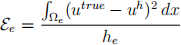
where and are the element domain and element length, respectively, for element e.

For each value of p (p = 1, p = 2 and p = 3):

– Plot the true solution, and the numerical solutions as Ne increases. Label each numerical solution by its degrees of freedom, DOF (number of nodes). The last plot should thus correspond to the DOF needed to reach the error tolerance specified above. Keep the figure axis somewhat tight to the true solution (e.g., to better see convergence of the solution as Ne increases to its final value, set axis([0 L -2 2])).

– Plot the final element error (x) over the domain.

– Plot a log-log convergence plot of error () versus element size (). Assuming = , estimate from this plot the convergence rate n. (Only use the linear portion in the loglog plot to compute convergence rate. This should occur as gets sufficiently small. Thus, you can estimate this from the last two mesh sizes.) Specify the convergence rate n on the plot (e.g. in the title).

Please ensure all plots have a title, axis labels, and legend labeling each plot.

Deliverables:

1. Thoroughly yet concisely describe the problem, how you solved it, and the results and interpretations. This can be typeset or a combination of very neat handwriting and computer-generated plots bundled in the order below.

(a) Introduction: Briefly describe the problem and goals (10pts)

(b) Method: Describe your solution strategy (PDE → Matrix equations) and computer algorithm (30pts)

(c) Results: Figures, Tables, etc. (10pts)

(d) Discussion: Interpretation of the results (10pts)

2. Matlab code (40pts)

All in all you will submit a PDF for item 1 and two Matlab .m files (Part 1 and 2) for item 2.

General programming guidance:

● Always sketch out your algorithm or pseudo-code before you actually start to program. This will clarify the big picture and information flow.

● Build your code in testable chunks. Do not try to do everything in first pass (e.g., do not worry about refining based on error, or generating all the plots, etc.). You can add in features as you become confident “core” components are working.)

● Comment as you go, not after the fact. That is, you should decide what you want before you do it, not after you do it.

● Learn how to use the debugger. E.g., use break points to see if variables are being updated as expected.

Assignment specific guidance:

● Create a function that will return Gauss weights and Gauss point coordinates:

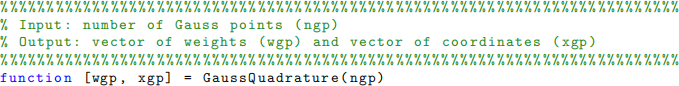
● Create a function that will return the local shape functions and shape function derivatives at an arbitrary x ∈ [−1, 1]. (You should call this function at your Gauss points.)

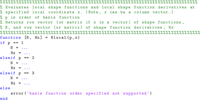
● The above functions can be called before the assembly loop.

● Your assembly loop over each element should have an inner loop over each Gauss point. (Thus, the stiffness matrix and force vector are built one Gauss point at a time.)

● You need to keep track of what nodes belong to what element (which is non-trivial for higher order elements or once we go to higher dimension). This is specified in a connectivity array (location matrix), which you need to generate.