FINA6532 FB & FC Quantitative Methods in Finance Assignment 3
Hello, dear friend, you can consult us at any time if you have any questions, add WeChat: daixieit
Assignment 3
FINA6532 FB & FC Quantitative Methods in Finance
Due: 14/11 (FB) & 15/11 (FC)
There are 100 points in total on this assignment. You may discuss your answers with other students, but please hand in your own assignment in your own words. Make sure to include your name and your student ID number. Late assignments will not be accepted. Subquestions qithin each question 1,2 and 3 are equally weighted.
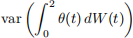
1 Itô Isometry (25 points) Find the variance of

using Itô isometry.
Note: do not use that  random variable, so that gives us that the variance is
  . You should, however, get the same answer. In your solution, feel free to push any expectations operators inside of any integrals.
2 Itô Integral (25 points) Let W be a standard Brownian motion. In this problem, I want you to compute

for two different adapted processes θ. This will give you some better insight for why you can get non-normal answers.
In this problem, sample paths of θ will always be constant on [0, 1) and [1, 2]. By that, I mean we will be considering processes where
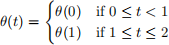
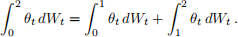
Note that this does not mean it isn’t random. It just means that You may want to use the fact that Itô integrals can be broken apart just like Riemann integrals:
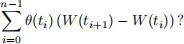
(a) Briefly explain why

There is no need to fully prove your answer. A simple argument is all you need.
Hint: for a partition t0 = 0 < t1 < · · · < tn = 1 of [0, 1], what is
(b) Suppose

Note that this is non-random. Calculate  . Express your answer in terms of W(1) and W(2).
(c) What is the distribution of  for the θ(t) in (b)?
(d) Now, suppose

Briefly explain why θ(t) is adapted.
(e) Find the variance
where θ(t) is as given in (d).
Hint: there are two ways to do it. You can condition on W(1), and use the law of total variance.
Or, you can use Itô isometry to do it much quicker.
(f) Sketch the density of  , where θ(t) is as given in (d).
Note: solving for the distribution requires some non-trivial integration. I’m not asking you to do that. Just sketch what the density will look like. As a hint, try to think about what happens when W(1) < 0 and W(1) ≥ 0, and then combine those.
3 Cox-Ingersoll-Ross Model (50 points) This is a different short-rate model to the one discussed in class. You will not be able to solve it using the techniques we have learned so far, but you can characterize the mean and variance with some tricks. Let

As with the Vasicek model, assume that a > 0. We will also assume that b > 0. It is also usually assumed that 2ab ≥ σ2 .
As a side note: in finance we call this Cox-Ingersoll-Ross model, because these authors used it to model the short-rate process. However, outside of finance this is called an Ornstein-Uhlenbeck process.
(a) Without do any math, briefly explain why rtwill remain non-negative? There’s no need for a formal justification.
Hint: look at the volatility. What happens as rt gets close to 0?
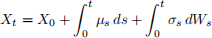
(b) Try the same trick as with the Vasicek model. That is, define Xt = eatrt, and use Itô’s Lemma to find the drift and diffusion of Xt.
Hint: make sure there is no rt in your expression (you will need to substitute it out). You should get something of the form dXt = µt dt + σt dWt, where µt depends only on time, and σt depends on time and Xt.
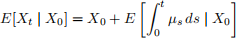
(c) What is the expected value E[Xt | X0]? Remember that the Itô integral is typically a martingale.
So, if you found dXt = µt dt + σt dWt, then
and therefore
(d) What is the variance var(Xt | X0)?
Hint: Remember the Itô isometry result. This gives you that
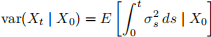
In this case, you should get something that looks like
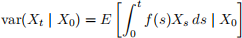
Push the expectation inside of the integral, and integrate. That is, switch the order of the integral sign and the expectation:
(e) Use your results to compute the mean and variance of rt conditional on r0.
Note: you can do this even if you couldn’t do all of (c) and (d). Just leave your answers in terms of E[Xt | X0] and var(Xt | X0) accordingly.
2023-11-27