Hello, dear friend, you can consult us at any time if you have any questions, add WeChat: daixieit

STAT 231 Fall 2021 Coursework 1

Assignment Component

The assignment component of Coursework 1 is due on Friday September 24th at 11:00am EDT. You may create your document in Word, Google Docs, LaTeX or any other word processor. The requirement to type your assignment is to facilitate the marking of hundreds of assignments so that the marked assignments can be returned to you in a timely fashion. It is also useful for you to gain some experience in creating a document containing mathematical expressions. Two documents have been posted in the Assignment 1 folder in LEARN on how to use the equation editor in Word. If you wish to use LaTeX then you may find Overleaf particularly useful for this. See https://www.overleaf.com/edu/uwaterloo  

Upload your assignment to Crowdmark as a pdf file for marking. You can upload your assignment as one document or individually for each problem. If you upload one document then you must drag and drop the pages for each problem to the appropriate question as indicated in Crowdmark. You can resubmit your assignment any number of times before the due time. Therefore, to ensure that there are no issues with uploading we advise you to upload your assignment well in advance of the due time. Assignments which are left as a single document and not uploaded to the appropriate places in Crowdmark will be assigned a 10% penalty.

Many problems on this assignment indicate that your written answers must be given in sentences. A overall penalty of 5% is applied to assignments which do not follow these instructions.

In this assignment you are asked to use R to answer some problems. The answers/results you obtain using R must be included in your Crowdmark pdf submission.  Additionally, the R code that you use must be uploaded as an R file to the appropriate LEARN Dropbox.

Effectively commenting your code is a really important skill to develop. Markers will review your file and run it to verify the answers match those in your Crowdmark submission and that the code runs without error. You code must correctly find the answers needed to get the marks associated with the problems. Good commenting will allow the marker to more easily assign you a full score when reviewing your file. Please ensure your code submitted in the R file is well commented.    

Checklist to complete for this assignment:

Upload the pdf of your assignment component of Coursework 1 to Crowdmark by the deadline. A penalty of 5% per hour is applied for late assignments.

Upload the R file of your assignment component to the appropriate LEARN Dropbox by the deadline. A penalty of 10% is applied if the R file is uploaded late or is missing.

Upload your data set, in csv format, to the appropriate LEARN Dropbox by the deadline. A penalty of 10% is applied if your data set is uploaded late or is missing.

This assignment is based on the material in Chapter 1 of the STAT 231 Course Notes.

Coursework 1 Assignment Component Learning Outcomes

Here are the intended learning outcomes for this assignment component. Try to identify the learning outcomes which are achieved by each of the given problems.

● Review properties of the probability models studied in STAT 230 and use R to determine probabilities for these distributions.

● Understand the basics of empirical studies such as approaches to data collection and types of variates

● Identify and understand the inherent variability about the expected results for graphical and numerical summaries across different samples for a fixed sample size

● Identify and understand the inherent variability about the expected results for graphical and numerical summaries across different sample sizes

● Compute and interpret numerical measures of location, variability, and shape for a data set

● Compute and interpret graphical summaries of data such as relative frequency histograms, empirical cumulative distribution functions, box plots, and bar charts

● Use numerical and graphical summaries to compare key similarities or differences between data sets

● Use numerical and graphical summaries to assess the fit of a specified probability model for the data

In Problem 1 you will review the Binomial, Poisson, Gaussian (Normal) and Exponential distributions which you studied in STAT 230. These distributions will be used extensively in STAT 231. As well you will use R to calculate probabilities for these distributions.

1.(a) Binomial distribution

In a very large population 1% of the people have a certain genetic mutation. Suppose 1200 people are selected at random. Define the random variable Y = number of people with the genetic mutation in the sample.

(i) Explain, with reasons, whether the Binomial model is a reasonable model to use for Y. (You may find it useful to review the setup for the Binomial model in the STAT 230 Course Notes.) Your answer must be written in sentences.

(ii) Type help(pbinom) in R to see the syntax for the R functions pbinom, qbinom, dbinom, and rbinom. Use the appropriate R functions to obtain values for:  

P(Y ≤ 8),      P(Y ≥ 16),    and   P(|Y – 12| < 7)

Use all the decimal places provided by R for your answers.

Be sure to include your commented R statements in the R file that you upload to the LEARN Dropbox.

(iii) Suppose the proportion of people with the genetic mutation is an unknown value equal to θ. Suppose n people are selected at random where n is large. Use the Central Limit Theorem to approximate the probability  

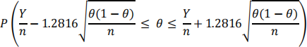
(You don’t need to use a continuity correction.) You must show your work for full marks.

1.(b) Poisson distribution

During the week of December 6‐13, 2020 the visits to an Eastern Ontario Health Unit website to book a Covid test occurred at random at the average rate of 10 visits per minute. Suppose it is reasonable to use a Poisson process to model this process. Define the random variable   Y = number of visits to the website in one minute.

(i) Explain, with reasons, whether the Poisson model is a reasonable model to use for Y. (You may find it useful to review the setup for the Poisson model in the STAT 230 Course Notes.) Your answer must be written in sentences.

(ii) Type help(ppois) in R to see the syntax for the R functions ppois, qpois, dpois, and rpois. Use the appropriate R functions to obtain values for:

P(Y < 5),     P(Y > 14),     and     P(|Y – 10| ≥ 7)

Use all the decimal places provided by R for your answers.

Be sure to include your commented R statements in the R file that you upload to the LEARN Dropbox.

(iii) Suppose Y1,Y2, …,Yn  is a random sample from a Poisson(θ) distribution and let  be the sample mean.  

Use the Central Limit Theorem to approximate the probability

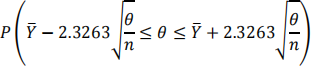
(You don’t need to use a continuity correction.) You must show your work for full marks.

1.(c) Normal or Gaussian distribution

Suppose it is reasonable to assume that the weights in grams of chicken eggs laid at a particular hobby farm have a G(60,9) = N(60, 81) distribution. Define the random variable Y = weight of a chicken egg chosen at random.

Be sure to include your commented R statements in the R file that you upload to the LEARN Dropbox.

(i) Type help(pnorm) in R to see the syntax for the R functions pnorm, qnorm, dnorm, and rnorm. Use the appropriate R function to obtain the value for:

P(Y ≥ 69)     and    P(|Y‐60| < 3)

Use all the decimal places provided by R for your answers.

(ii) Use the appropriate R function to obtain the value for a such that P(Y ≥ a) = 0.87. Use all the decimal places provided by R for your answers.

(iii) Suppose 100 chicken eggs are chosen at random. Determine the probability that their average weight lies between 59 and 62 grams. Use R to find the probability, not the Normal table in the Course Notes. Use all the decimal places provided by R for your answer.

You must show your work for full marks.

1.(d) Exponential distribution

Suppose it is reasonable to model the battery life (in hours) of a certain type of watch battery using the Exponential(3) distribution. Define the random variable Y = battery life (in hours) of a randomly chosen watch battery.

(i) Explain, with reasons, whether the Exponential model is a reasonable model to use for Y. (You may find it useful to review the setup for the Exponential model in the STAT 230 Course Notes.)  

Your answer must be written in sentences.

(ii) Determine the median of this distribution, that is, determine the value m such that  

P(Y ≤ m ) = 0.5

You must show your work for full marks.

(iii) Type help(pexp) in R to see the syntax for the R functions pexp, qexp, dexp, and rexp. Use the appropriate R function to obtain the value for P(Y ≥ 4). Use all the decimal places provided by R for your answers.

Include the R statement that you used in your R file that you upload to the LEARN Dropbox.

(iv) Suppose Y1,Y2, …,Yn  is a random sample from a Exponential(θ) distribution and let  be the sample mean.  

Use the Central Limit Theorem to approximate the probability

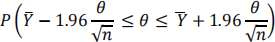
Use R to find the probability, not the Normal table in the Course Notes. Use all the decimal places provided by R for your answers.

You must show your work for full marks.

Include the R statement that you used in your R file that you upload to the LEARN Dropbox.

2. Empirical Studies

The purpose of this problem is to examine how empirical studies are reported in the news media.

On the course website on LEARN you will find a module under Additional Resources called Statistics in the Media. These are all examples of empirical studies which have been reported in the news media.

Find your own example of statistics in the news media. You may not use an article from the course website.

News media includes print media (newspapers, newsmagazines), broadcast news (radio and television), and the Internet (online newspapers, news blogs, news videos, live news streaming, etc.).

Pick a topic which is of interest to you and search online using keywords which describe your topic.

Your example must be less than 2 pages long.

Your article must not come from a research journal. An article in the news media based on an article in a research journal is okay.

Make sure you chose an example for which the data are a sample of a larger population and not a census of that population.

The example must have appeared in the news media after August 31, 2020.

(a) Indicate clearly the information on where the article appeared and the date it appeared. Give the link to the article. To help the TAs mark this question please cut and paste the article into your assignment.  

The answers to (b) ‐ (f) must be written in full sentences.

(b) Give the keywords you used to find your example and explain why this topic is of interest to you.

(c) State clearly and succinctly what the purpose of the study was and the conclusion reached by the researchers.

(d) The study you selected can be best described as which of the following: an observational study, a sample survey or an experimental study? Justify your answer.

(e) What are the units in this study? Based on the given information, what population or collection of units are the researchers interested in?

(f) Give the 2 most important variates in this study and indicate the type of each.

In Problem 3 you will investigate the behaviour of numerical and graphical summaries for different samples which are randomly generated from the Negative Exponential models using the R shiny app:

https://shiny.math.uwaterloo.ca/sas/stat231/datasummaries/

All written answers must be in full sentences.

3. Negative Exponential

(a) The probability density function of a Negative Exponential random variable is  

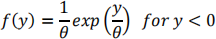
and 0 otherwise.  

Determine the mean, median, standard deviation and cumulative distribution function for this distribution. You must justify your answers.

(Hint: Note that W = ‐Y has an Exponential (θ) distribution.)  

(b) Briefly describe what you would expect the sample mean, sample median, and sample standard deviation to be for a randomly generated sample from this distribution if θ = 2.

(c) Click on the link to the R shiny app. Select the Negative Exponential(θ) distribution and change the parameter to θ = 2. Select the number of bins to be 10. Select a sample size of 100. Click the Resample! button 5 times and enter the values for the sample mean, sample median, and sample standard deviation for each of the 5 samples in a table such as the following.

Sample	1	2	3	4	5
Sample mean
Sample median
Sample standard deviation

(d) By looking at the table, summarize the behaviour of the sample mean, the sample median, and the sample standard deviation for a fixed sample size.

(e) Select a sample size of 500 and the number of bins to be 12. Click the Resample! button 5 times and enter the values for the sample mean, sample median, and sample standard deviation for each of the 5 samples in a table such as the one in (c).   

(f) Repeat (e) for a sample size of 1000.

(g) By looking at the three tables, summarize what happens in general to the sample mean, sample median, and sample standard deviation as the sample size increases.

(h) What do you notice about the shape of the empirical distribution function as the sample size increases?

Further practice:

To gain an understanding of the variability that you might expect in data sets generated from different distributions we strongly recommend that you use the R shiny app to investigate the other distributions available which include the Gaussian, Uniform, Exponential, and t distributions.

In particular you should notice how numerical and graphical summaries vary from sample to sample for a fixed sample size and how numerical and graphical summaries vary as sample size increases.

In Problems 4 and 5 you will begin to analyse the Twitter data set that will be used in this course.

See the document called Assignment Dataset Information posted on LEARN (Content ‐> Submissions ‐> Coursework Submission 1) which includes a description of the data set and information on how to download your data set. See also Assignment 1 R Tutorial (pdf document) and 231_R_Tutorial (video) posted in the same folder which includes information which will aid you in creating your own code for doing these problems.

All written answers must be in full sentences.

Example:  

The variate day.of.week is a __________ variate.  

4. Day of week of tweet

In this problem you will examine the data for the variate day.of.week (the day of the week the tweet was published on Twitter) for two of your 3 chosen personal accounts.

(a) What type of variate is day.of.week?

(b) From the 3 personal accounts you have chosen for your data set, select two.  

(i) Provide a frequency table and a bar graph for the day.of.week variate for each of these two personal accounts. The table and graph must be arranged in the order of the days of the week (Monday to Sunday).

Be sure to label your table and graph.

(ii) What is the sample mode for the day.of.week variate for each of these two personal account, in other words, what is the most popular day of the week for tweets for each of these personal accounts?

(iii) Is the distribution of the day.of.week variate similar for both accounts? Justify your answer.  

Be sure to include your commented R statements in the R file that you upload to the LEARN Dropbox.

5. Time of day of tweet

In this problem you will examine the data for the variate time.of.day (the time of day the tweet was published, expressed as seconds after midnight) for the two organization accounts you chose for your data set.

(a) What type of variate is time.of.day?

(b) Complete the following table for the time.of.day variate for your two chosen organization accounts. Numbers may be rounded to 3 decimal places. Change the titles to the usernames of your chosen accounts.

	Username of Organization 1	Username of Organization 2
Sample mean
Sample median
Sample standard deviation
Sample skewness
Sample kurtosis

(c) For each of your chosen accounts create and insert the plot of the relative frequency histogram with superimposed Gaussian probability density function.

All plots must have titles and axes labelled appropriately to receive full marks.

(d) For each of your chosen accounts discuss how well the Gaussian model fits the data. Use the graphical and numerical summaries to justify your answer. You should make at least four comparisons between what you observed for your data set and what you would expect to observe if the data were generated from a Gaussian model.

(e) Provide a side by side boxplot for your two chosen accounts.

Suppose you were only given this boxplot. Describe the information about the differences and similarities between the 2 groups of data that you can obtain just from this plot. Things you might wish to comment on include:  

● a comparison of the symmetry of the data sets

● a comparison of the tail regions of the data sets

● a comparison of the ranges (variability) of the data sets

● a comparison of the medians (location) of the data sets

● a comparison of the number of outliers of the data sets

Be sure to include your commented R statements in the R file that you upload to the LEARN Dropbox.