ENG2106 – Numerical and Statistical Methods Assignment 2
Hello, dear friend, you can consult us at any time if you have any questions, add WeChat: daixieit
ENG2106 – Numerical and Statistical Methods
Assignment 2: Programming Application
1. Key information
|
Module name |
ENG2106 - Numerical and Statistical Methods |
|
|
Unit of Assessment |
Assignment 2: Programming Application |
|
|
Unit of Assessment weighting
|
30% |
|
|
Submission date |
24 November 2023, 4 pm |
|
2. Learning Outcomes
By completing this coursework you are demonstrating your progress on the following of the module’s learning outcomes:
1. Use MATLAB and programming as a tool to help solving Civil Engineering relevant problems.
2. Move towards independent research, application and analysis of numerical methods for engineering problems.
3. Convey technical information in a written report to a professional standard.
3. Tasks
This coursework consists of two tasks where you need to demonstrate your MATLAB skills, when applying numerical methods taught in the class, in real Civil Engineering problems. You should complete all tasks and write the results up in the form of a report. The report must include a brief description of how you approached each task, all the code that you used to complete the tasks, as well as the relevant outputs, e.g., figures and other numerical output. The coursework should be submitted as a single pdf-file through the Assignment folder on SurreyLearn.
Conciseness in explanation and presentation is important, and the whole report does not need to take more than 10 pages. However, if you do not manage to meet this limit, you should prioritize being complete, clear and correct over being concise and sticking to the page limit.
Task 1. Dynamic response of a damped oscillator (60 points)
Consider the spring-damper-mass system of Figure 1.
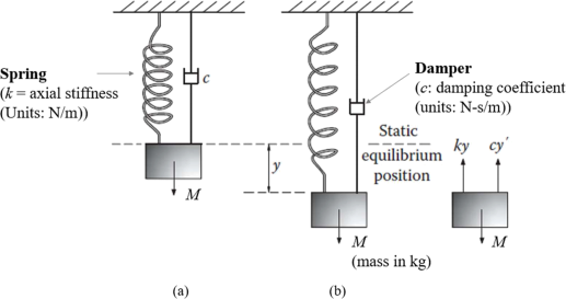
Figure 1 The oscillator of interest (Spring-damper-mass system): (a) in static equilibrium;(b) at a random displacement (vertical distance) from the static equilibrium position of (a)), as this is represented by the variable y (in meters).
The system is shown in Figure 1(a) in its initial resting position, after it has reached static equilibrium under its own weight’s action. In Figure 1(b), the system is shown at a random position outside its resting position. As it can be seen in the latter figure, the variable that represents the vertical displacement from the resting position is y, which is the dynamic displacement of the system, since it refers to its dynamic motion, i.e., its motion as a function of time, t. The mass of the body is represented by the variable m. The axial stiffness of the spring that holds the system hanging is k. During oscillation about its resting position, there is an inherent mechanism of the system that absorbs kinetic energy and transforms it to different types of energies, which eventually damp out the oscillations. The capability of the system to absorb kinetic energy and eventually stopping vibrations, as per the above scenario, and which can be caused by any type of external excitation, e.g., external forces or external imposed displacement, is usually, generically termed damping. The actual mechanism of damping, i.e., the mechanism through which a system absorbs energy and transforms it to other types of energies (in this case from kinetic to thermal, and other types), can be unknown in many cases.
However, in structural dynamics, and in dynamics of systems, in general, this capability is quantified through a quantity called damping constant or damping coefficient, which is usually represented by the variable c. The damping coefficient expresses the amount of energy transformation/absorption per cycle of motion of the system, where one cycle of motion is the motion of the system to move from one position, back to this initial position, after undergoing a full free vibration.
The equation of motion of a viscously damped system under the above so-called free vibration (i.e., the motion the system is left to vibrate after being initially excited, and left without any further, continuous, external force applying on it) is given by the following mathematical formulation (Ch. 2 of Chopra (2019)):

where, y(̈) and y(̇) are the second and first derivatives, respectively, of the vertical displacement beyond the static equilibrium position, y, as per Figure 1. As known, the second derivative of the displacement refers to acceleration, and the first in the velocity of the system.
As it is the case in the discipline of Structural Dynamics, the above equation of motion is usually solved numerically, given the wealth of numerical methods that have been proposed and developed for such applications.
Subtasks of the problem
Based on the description of the system, you are required to obtain the following subtasks:
a. Develop a code in MATLAB, utilising the classical 4th order Runge-Kutta Method (RK4), whereby you can estimate and visualise (graphically, i.e., through plots in MATLAB) the response of the body of the system over the time, t. The response refers to the motion, i.e., the dynamic displacement and velocity of mass, m, as a function of time, t. The program to be developed, should be enabling its user, i.e., the engineer, to input values for the characteristics of the system (m, k, c, t), and for an imposed initial displacement, from their ‘keyboard’. Mind that the initial, imposed displacement will represent the cause for the subsequent free vibration the system will undergo, and so, it will serve as the initial external loading of the system (but in this case, in terms of system deformation). Note that the initial static displacement of the system, i.e., the vertical displacement that has been caused by the application of the mass on the unstretched spring (spring with no mass at its lower end), can be ignored. For this task, you are only required to provide the code, without any actual plots (20 points).
b. Utilising the code of (a), you are required to now plot, in the same figure, the system’s displacement and velocity response over a time period of 20 seconds (integration domain), as a result the mass being pulled 3 meters below its resting position (so, its initial imposed displacement would be 3 meters). For your solution, consider the following values for the characteristics of the system: m = 30 kg; k = 150 N/m; and c = 3 N-s/m (5 points). For your initial conditions, you can also assume that the velocity of the system, when the body has been pulled at its initial vertical displacement of 3 meters, is zero. In the plots, you will need to plot the final values of the displacement and velocity at the end of the 20 seconds (e.g., with introducing markers, accompanied by relevant values, inside the plots)) (5 points).
c. Develop a code that has the same objectives with Sub-task (a), but this time with utilising the ode45built-in function of MATLAB, instead of utilising the RK4 method (20 points).
d. Then, apply the same input values with (a) in the code of (c), and plot the responses of the system (displacement and velocity over time), for the same period (20 secs). Also, plot in the graphs, the final values of the velocity and displacement at the end of the time domain, similarly with what you did in (b) (5 points)
e. Based on the results of (b) and (d), comment on any likely observed differences in the final values of the response (i.e., that at the end of the 20 seconds), as these may arise (if applicable) from the utilisation of the two different methods the associated codes employ. Justify your observations and comments, based on the concepts the two different methods draw upon (10 points).
Task 2. Mode shapes of a 3-storey building structure and fundamental frequency (40 points)
Consider a three-storey building structure. The building is symmetric and is expected to remain elastic and linear under its design loads (both vertical, .e.g., gravity, and horizontal, e.g., winds and earthquakes). Based on this, and within the framework of structural dynamics, the horizontal response of the structure, which is usually the most troublesome to be derived, can be determined assuming that the second order differential equations of motions can be decoupled and simplified. The dominant method in doing this, is the so-called modal analysis (See Chapter 10 of Chopra (2019)). For this to be realised, the basic step is to derive the so- called mode shapes of vibration of the structure, or more simple, its mode shapes. The latter, in turn, necessitate that the eigenvectors of the structure are derived. In structural dynamics, these vectors, which is a special type of vectors, form the so-called eigenmodes (see also Ch. 27 of Chapra and Canale (2015)).
For the structure, the mass matrix, M, and the stiffness matrix, K, are given in Figure 2, next. Based on these, you can proceed with the sub-tasks that are asked from you next.

Figure 2 Mass and Stiffness matrices for the three-storey structure
The elements in the Mass Matrix are in kN-sec2/m units, while those in the Stiffness Matrix are in kN/m units.
For this task, you will be required to do the following sub-tasks:
(a) Create a program in MATLAB for calculating the mode shapes of the structure, utilising the method of Modal Analysis. The program shall enable the user to input the mass and stiffness matrices from their keyboard. The units for the associated mass and stiffness values to be introduced in the aforementioned matrices should be presented to the user before they input these values in the program. Also, the program should enable the user to derive the fundamental frequency of the structure (20 points).
(b) Based on the matrices given in Figure 2, calculate the mode shapes and the eigenvectors of the structure. Plus, determine the fundamental frequency of the structure in appropriate units (10 points).
(c) For the results of (b), normalise the mode shapes, and sketch their profiles (10 points).
4. Marking Criteria
Each of the two tasks will be marked separately, with reference to the University Grade Descriptors on three criteria:
1. Correctness of results (40%).
2. Quality of the MATLAB code (45%).
3. Presentation of the report (15%).
The two tasks of this assignment carry different weights: Task 1 carries 60% of this assignment’s total grade, and; Task 2 carries 40% of the total weight of this assignment. Their weights reflect the complexity of the work involved in each task.
Correctness of results is demonstrated by:
- You implementing the functions and scripts correctly and hence presenting the correct, anticipated results.
- You use to-the-point and correct language when discussing your approach to each question.
- Correct and consistent use of equations and terms.
Quality of MATLAB code is demonstrated by:
- Correctness, readability and conciseness of the code.
- The appropriate use of comments.
- The use of MATLAB techniques introduced in the lecture notes and tutorials. In particular, these are: the use of scripts and function.
- Where appropriate, it is preferred to develop generic and reusable solutions, based on the concept of the user-defined functions of MATLAB. See also Section 8 of the Introduction toMATLAB lecture notes.
The presentation of the report will be expected to be professional, which includes the following:
- Title page including your URN.
- Consistent numbering of sections, pages, equations, tables, and figures.
- Consistent use of styles (fonts and sizes) for headers and body text.
- Well-formatted and appropriately sized figures and tables.
- All figure axes labelled. A descriptive caption for each table and figure.
- Well-formatted and numbered equations.
- Correct and to the point language (be concise).
- Inclusion of a reference section and correct use of references and citations using the Harvard system.
- The style and formatting must be consistent over the whole report and not vary per question.
5. Feedback opportunities
Please make use of the Discussion forum and tutorial sessions, if you have any questions about the use of MATLAB, or about possible, supplementary resources that may be required to support the research-led demands of this assignment.
6. Any specific conditions
All work must be done by yourself. The usual rules for plagiarism, citation and attribution apply and also extend to the use of MATLAB code. If you are at some point inspired by code from an external source, this must be clearly indicated, referenced and justified in the written report. Any failure to do so will be referred to the Department’s Academic Integrity Committee.
Any externally inspired code must be fully adapted to the standards and techniques used and recommended in the module. In other words, you have to make it your own. Any failure to do so will result in the lowest possible marks for Quality of Results and Discussion and Quality of MATLAB Code.
7. Sample feedback form
Feedback will be provided using the form shown in Figure 2 (note the values in this table is just an example).
8. References
Chopra, Anil K. (2019), “Dynamics of Structures in SI Units”, 5th Edition, Pearson Education Limited.
Chapra, Steven C., and Canale, Raymond P. (2015), “Numerical methods for engineers”, 7th Edition (International Edition in SI units), McGraw Hill.
2023-11-23
Programming Application