SOCI 411 – Fall 2023 SYNTAX EXAMPLES FOR LAB ASSIGNMENT #4
Hello, dear friend, you can consult us at any time if you have any questions, add WeChat: daixieit
SOCI 411
Fall 2023
SYNTAX EXAMPLES FOR LAB ASSIGNMENT #4
*Note: These examples were created using the GSS27 survey data.
Running a crosstab of two variables, each with two response categories and calculating and interpreting chi-square and phi. (Questions 2-4)
First, doing appropriate recodes and stating hypotheses.
*Note: For my analysis I need to recode the variable PRCODE (province of residence) to make it a two category variable – this is my Independent Variable. Ido not need to
recode the variable VBR_10 (voted in last federal election) as it only has two categories – this is my Dependant Variable. Below I pasted the syntax for my recode and ran
frequency distributions of the variable before and after recoding. I posted the output for both my original and recoded variables below along with the syntax.
FREQUENCIES variable PRCODE.
recode PRCODE (46=1) (47=1) (48=1) (59=2) (10 THRU 35 = 2) into newREGION. missing values newREGION (96 THRU 99).
value labels newREGION 1 'Prairies' 2 'not Prairies'.
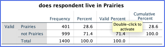
variable labels newREGION 'does respondent live in Prairies '.
freq var PRCODE newREGION.
Original variable output:

Recoded variable output:
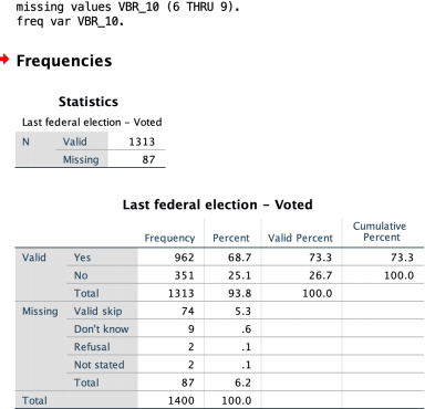
My second variable VBR_10 does not need to be recoded. The frequency and syntax are pasted below.
missing values VBR_10 (6 THRU 9).
freq var VBR_10.
My hypotheses are as follows (I have used a non-directional research hypothesis, but you can also use a directional hypothesis if the question does not specify):
H0 : The proportion of people who have voted does not vary by region (i.e., Prairies
versus not in Prairies). In other words, there is no relationship between the region that one resides in and voting behaviour.
Ha : Voting behaviour will differ based on the region people reside in (i.e residing in the Prairies versus those who reside outside of the Prairies).
Now, running a crosstab of the two variables and describing the output.
Crosstabs tables = VBR_10 by newREGION
/cells=column count
/statistics = chisq phi.

From this crosstab we see that 64.3% of people in the prairies voted in the last federal election, as compared to 76.8% of people who do not live in the prairies.
So far, this supports my research hypothesis, as a higher proportion of people who reside in the Prairies have not voted as compared to those who do not reside in the Prairies.
However, while there appears to be a difference in voting across region based on this sample data, we cannot make any conclusions yet until we run a hypothesis test via the chi-square test.
Tesing statistical significance and strength of the relationship in a 2x2 table using chi square and phi.

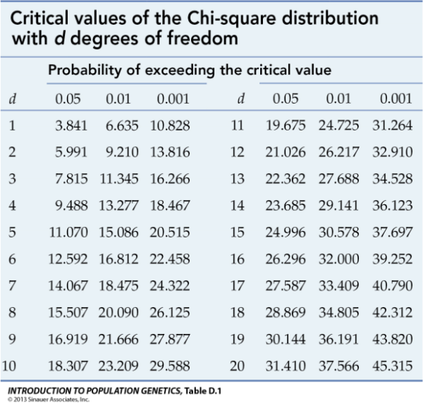
The chi-square value/statistic obtained is 21.185, well above the critical value of 3.841 for a 2x2 table. Therefore, we can reject the null hypothesis of no relationship between region and voting behaviour. Here, the value of Phi is at -.127 so the relationship is
weak. We conclude that the relationship between region and voting behaviour is significant but weak.
Running a crosstab of two variables, but replacing one variable from the previous example with a different variable that has 3-5 valid responde categories.
Calculating and interpreting chi-square and Cramer’s V. (Question 5)
*Note: We will be testing the relationship between DH1GED (educational level – the IV) and VBR_10 (voting behaviour – the DV). First, we must state our hypotheses. I already ran a frequency for VBR_10 above, so now I am just running a frequency table for
DH1GED. My hypotheses are also stated below:
*Syntax:
FREQUENCIES variable DH1GED.

H0 : The proportion of people who have voted does not vary by educational level.
Ha : The proportion of people who have voted does differ by educational level.
Now, running a crosstab of the two variables and describing the output.
Crosstabs tables = VBR_ 10 by DH1GED
/cells=column count
/statistics = chisq phi.
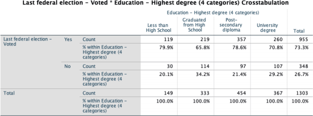
From this crosstab, we do not see a consistent trend related to highest degree obtrained and voting behaviour but there does appear to be a relationship between our two
variables. Those with less than a high school degree were most likely to vote (at 79.9%),
followed by those with a post-secondary degree (at 78.6%), those with a university degree (at 70.8%), and those with a high school diploma (65.8%). Thus, we see
differences across categories of the IV but no consistent positive or negative trend.
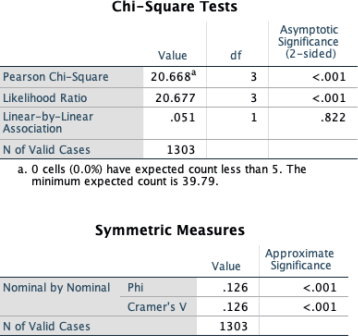
The chi-square value obtained is at 20.67, well above the critical value of 7.815for a 2x4 table (DF = 3, p<.05). Therefore, we can reject the null hypothesis of no relationship
between education level and voting behaviour. Here, the value of Cramer’s V is at .126 so the relationship is weak. We conclude that the relationship between education level and voting behaviour is significant but weak.
Use one of the previous cross-tab examples examined and consider a third variable using the elaboration method (Question 6).
*So using the original syntax and table above that examined region of residence and
voting behaviour, I will now be adding sex as a third variable to extend the relationship between two variables into an elaboration model.
Now, we will be taking into account—or controlling for—respondent’s sex (our Z variable) in examining the relationship between region (X) and voting behaviour (Y). Sex is an ANTECEDENT variable in the relationship between X and Y.
Crosstabs tables = VBR_10 by newREGION by Sex
/cells=column count.

Analysis for elaboration model:
The original zero-order relationship between voting behaviour and region is shown
previously. To reiterate, the original relationship shows that 64.3% of people reside in
the prairies voted in the last federal election, as compared to 76.8% of people who do not reside in the prairies,for a 12.5% difference.
However, the inclusion of respondents’ sex into the model allows us to control for
whether someone has identified as female or male. Within the subgroup of respondents who identified as males and have voted in the last federal election, we see that 61.8%
reside in the prairies compared to 77.1% of those who do not reside in the prairies,for a 15.3% difference. This shows a difference once controlling for sex, in which the partial
relationship for males is stronger compared to the original relationship (12.5% difference for original; 15.3%for partial relationship).
Within the subgroup of respondents who identified asfemales and have voted in the last federal election, we see that 66.8% reside in the prairies, compared to 76.6% who did not reside in the prairies,for a 9.8% difference. According to the percentage difference, the partial relationship for females is weaker compared to the original relationship of
region and voting behaviour (12.5% difference for original; 9.8%for partial relationship)
The analysis shows that the relationship between voting behaviour and region of
residence is affected by respondents’ sex. The relationship between voting behaviour
(specifically those who have voted) and region is more pronounced for males. On the
other hand, the relationship between voting behaviour (specifically those who have
voted) and region is weakened for females. This indicates specificiation occurred, as we see an increase in one group of Zand a decrease in the other.
Running and interpreting a scatterplot and Pearson’s R for two interval/ratio variables. (Questions 7-10)
*Note: Although not shown in this example, remember to always start by running a frequency of your variables so that you know what they are measuring.
H0 – There is no relationship between hours worked per week and a respondents number of close friends.
Ha (non-directional) - There is a relationship between hours worked per week and a respondents number of close friends.
Ha (directional) – There is a positive relationship between hours worked per week and number of close friends (as you work more hours, you will have more close friends).
The IV is hours worker per week and the DV is number of close friends.
graph
/scatterplot= WHW_120C with SCF_100C.
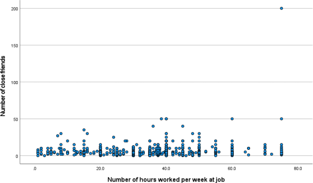
Visually, it is hard to interpret the trend in this data. It looks to have a very weak positive linear association.
correlations
/variables = WHW_120CSCF_100C
/statistics descriptives.
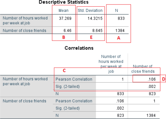
A) Sample Size: The sample size was 833 people for the variable on hours worked, and 1384 people for the variable on number of close friends.
B) Mean: The mean hours worked per week is 37.27 and the mean number of close friends was 6.46
C) Association: The Pearson’sR value is significant at the level of p<.01. The
Pearson’sR value is positive and weak at 0.106. This means that there is a significant positive but weak association between hours worked and number of friends – people with MORE hours of work are associated with HIGHER number of close friends on average. This does support my analysis of the
scatterplot and the directional hypothesis I made (!). NOTE:THIS MAY NOT ALWAYS BE THE CASE!
D) R2 = 0.011 (0.106*0.106). This means that the error in predicting number of friends is reduced by 1.1% if we know how many hours a week a person
works.
E) SD. The standard deviation of number of hours worked per week is 14.32 and of number of friends is 8.64. Using r we can state that a one SD increase in
number of hours worked per week is associated with a 0.106 SD increase in
number of close friends. In numbers, a 14.32 unit increase in number of hours worked per week is associated with a 0.916 (8.645 * 0.106) increase in
number of close friends.
Running and interpreting a Spearman’s Rho for the same interval/ratio variables as above.
Nonpar corr
/Variables = WHW_120CSCF_100C
/print = spearman.
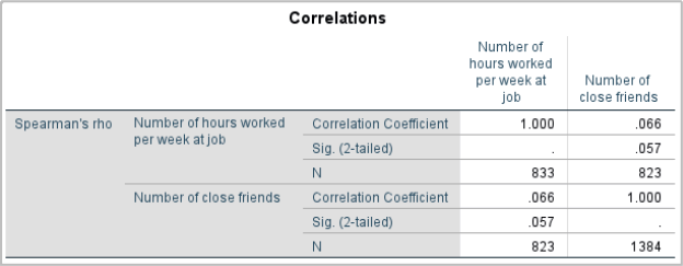
SPSS finds that the rank-order Spearman’s rho correlation between the two variables is 0.066. We therefore find a a weak positive correlation between number of hours worked per week and number of close friends. Knowing the rank on number of hours worked per week reduces the error of predicting the number of close friends by 0.4% (0.066 * 0.066). However, we can also see that the correlation is NOT statistically significant at 0.057
level with p>.05. NOTE: Since this result is NOT significant, we would not normally
include the interpretation of this coefficient. This has been included merely to exemplify how you would interpret a significant finding.
2023-11-23