Hello, dear friend, you can consult us at any time if you have any questions, add WeChat: daixieit

ECE 514 Project: Part 2

Setting Clipping Levels for Speech Signals

Good performance of audio communication over a telephone line channel hinges on the quality of the signals (speech and music) and hinges on minimizing ”clipping” of signals by the receiver am- plifiers (i.e. limit the magnitude of signals). Clipped speech sounds-caused distortion is often found objectionable. The amplitude of audio/speech is commonly modeled by a Laplacian Prob. Density Function (PDF) [Rabiner and Schafer 1978]. As maybe seen, the amplitudes are concentrated near zero, and the likelihood of larger ones is according the following,

As illustrated in Fig.-1, the width of the PDF is an increasing function of σ2. This parameter σ2 plays in effect the role of variance of the PDF as well as reflects the signal power (e.g., speech in this case).

Figure 1: Laplace distribution PDF for various σ2  values

Guarding against an excessive clipping is ensured by keeping the signal magnitude within a pre-determined level regardless of the likelihood of the event. Imposing such a no-clipping requirement on the electronics to 99% of the time might be one case. A model for a pre-clipper, as shown in Fig.-2, would avoid any distorting saturation by the amplifiers so long as the input signal magnitude is within the interval −A ≤ x ≤ A, thus limiting the maximal positive/negative amplitude to +A for any signal magnitude exceeding | A |.

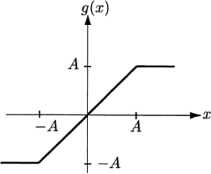
Figure 2: Clipper input-output characteristics

Assuming the input signal amplitude Laplace-distributed per above, and we can observe discrete samples of the input and of the regularized-clipped signal.

1.  For a clipping transformation level of A, derive an expression for the probability of clipping, Pclip , where

Pclip  = P[X > A  or  X < −A]

2.  Suppose now that Pclip  is bounded above at a certain value (say 0.01, i.e.  the input signal getting clipped at most 1outof 100 samples on average, not more frequently than this rate). Derive an expression for the clipping level, A in this case.  (HINT: In other words, find the maximum allowable magnitude of the signal amplitude, so that it is not clipped at a rate above Pclip ).

3.  How does A change as the signal power, σ2  is increased?

4.  What is the expression of the CDF, FX (x) for the Laplace distribution with a PDF defined in Equation-1.

5.  Using the inverse of FX (x) derived above, generate discrete input samples from the Laplace distribution. Use the values, σ2  = 1W.

6.  Plot 50 such samples (example plot of input samples shown in Fig.-3).  Assume Pclip   = 0.01. How many samples do you estimate would be clipped? Does your plot agree with the estimate?

7.  Suppose now that a single speech signal is sensed by a microphone in a noisy environment, e.g., a concert hall with N attendees. Assume that there is a single singer on the stage besides the N attendees so that one models the sensed signal as

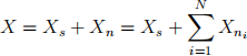
where Xs  is the signal from the main source of interest and Xni   are the background ”noise” signals.

We assume that the Laplace distribution model governs all the signals, with however the main source Xs  and the remaining auxiliary sources will respectively have a variance of σs(2) and {σn(2)} (for each of the N auxiliary sources) and σs(2)  >> σn(2)  due to the proximity to the microphone.

8.  What will be the PDF of Xn if N is very large? Justify your explanation.

9.  What will be the average power of Xn?   Explain mathematically how this power would change as N is increased.

The clipper amplifier was designed for a clipping level of 20 V (i.e.  A  = 20V) with an acceptable Pclip   =  0.01.  If σn(2)  = 0.001W, σs(2)  =  1W, what is the maximum number of concert attendees, N to ensure that the actual clipping likelihood remains below Pclip?

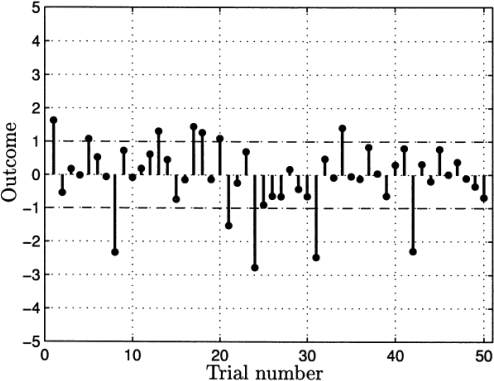
Figure 3: Clipper input-output characteristics