MMB8048 – Data Analysis Experience: Analysis of data from Houldcroft et al 2016
Hello, dear friend, you can consult us at any time if you have any questions, add WeChat: daixieit
MMB8048 - Data Analysis Experience: Analysis of data from Houldcroft et al 2016
AIM: Use bioinformatics tools available on the internet to analyse data from Houldcroft et al.
OUTCOMES:
• gain an insight to the complexity of extracting and analysing next generation sequence data.
• appreciate the power of NGS analysis with the right clinical samples.
INTRODUCTION: The Houldcroft et al paper describes how they used next generation
sequencing (NGS) to identify the propagation of drug resistant viral variants in a cohort of paediatric patients. NGS was able to identify mutations that conventional PCR based
diagnosis methods were either unable to detector were not sensitive enough to detect. Their analysis showed, retrospectively, that the clinical outcomes correlated with the
appearance of known and novel genetic variants in 3 genes that conferred resistance to the drugs used to treat the patients in question.
I have heard the senior author discuss this work at a NGS symposium asking “What can whole genome sequencing do for clinical and public health microbiology.” Her talk on this topic and the resulting debate was one particular highlight for me which is why I have
chosen the paper as course material.
This paper allows us to explore another impact of NGS rather than just bacterial
identification. Here we focus on viral genetics and the importance to identify and track genetic point mutations, known or new, associated with drug resistance, especially in cases of prophylactic treatment.
There are key steps in our analysis that will not happen instantaneously and depending on the system we will use they may work or not within our time window!
What we need to do: I have divided this experience in to three phases. The aim being to exploit these sessions to provide you with the key information to perform the analysis
pipeline we require to achieve our objective.
Phase 1: Introduction to our analysis pipeline, confirm everyone has access to the
necessary software, discuss the paper as a group, and begin our analysis by focusing on the genes UL54 and UL97
Phase 2: The authors description of UL97 can really exemplify the power of the type of
analysis and is visually noticeable once we get to seeing our own results. Therefore, in this
phase we will learn how to approach the analysis with a focus on UL97. We will then exploit our new skills by repeating the extract of UL54 data from the NGS data set.
Phase 3: Visualising the data in our own format. We will focus on analysing the data we
have extracted to represent Figure 1 and 3 using our own output. Using this analysis is the basis of your report.
The above will take quite a few specific steps:
Phase 1:
1) Identify the UL97 DNA sequences from the reference genomes and download them in FASTA format.
2) Repeat step 1 for UL54
3) Generate baseline alignments and phylogenetic trees of the reference data.
Phase 2:
4) Access the NGS sequence data for "Patient B" from the study.
5) Map the NGS sequence data to UL97 using an alignment tool known as BOWTIE2 . 6) Visualise the mapping results using the IGV software [Key to appreciate the data]. 7) Repeat steps 5/6 for UL54
Phase 3:
8) Extract the necessary data to reproduce figure 1 findings
9) Extract the consensus sequence from the BOWTIE2 alignments.
10)Integrate the consensus sequences into the reference alignments and phylogenetic trees.
11)Compare our outputs to the description of the analysis in the paper.
Phase 1
1) Identify the UL97 DNA sequences from the reference genomes and download them in FASTA format.
Website:https://www.ncbi.nlm.nih.gov/
Method: In the papers methods section under phylogenetic analysis you will find a list of
accession numbers. Use the link above to navigate your web browser to the NCBI website. Choose the database 'nucleotide' from the very long list next to the search box.

Type in the first genome number. This should bring up just one file. If so click on the 'Graphics' link (take a few moments to look at the genome):

In the search box search for UL97 and double click the search result. This should zoom in to the UL97 gene. Hover over the gene and a popup list will appear. Click on either
'FASTA VIEW.' Next in the top right corner click on 'send' choose 'file' and this will then download the FASTA sequence as an ASCII text file to your download folder (note the name of the file and the genome you are working with!) .
Repeat this for all 11 reference genomes. I will warn you at least one accession number is wrong! How would you search for the complete genome? Can you overcome this mistake yourself?
2) Now repeat this process for UL54.
3) Generate a baseline alignment and phylogenetic tree of the reference data
Method: We are going to go back to the downloaded FASTA files. Using word or a text editor create a new file with the following lines:
>UL97_Merlin
>UL97_[Viral_Strain] one for each viral strain used as a reference.
You will then need to copy paste the DNA sequence from each downloaded UL97 fasta file in between the > lines:
>UL97_Merlin
DNA SEQUENCE
>UL97_xxx
DNA SEQUENCE
Save this file as UL97_ref.fasta in text format.
We are going to use the MEGAX platform to analyse the data.
We will need to first install MEGAX on you computer. I will walk you through this but it should be quiet straightforward whether you are on a PC or a MAC.

Open MEGAX and using the tabs available choose "Align" > Edit/Build Alignment. In the new "Align" window now choose "Data" > "Open" > "Retrieve sequences from file" directing MEGA to the file UL97_ref.fasta.
This now allows you to run a multiple alignment using CLUSTAL or MUSCLE using the pulldown menu "Alignment". Make your choice which you use noting it down in your notebook, leave everything as default and click "compute".
You will then need to export your alignment as a .meg file.
Go back to the first window and via "Data" > "Open a File/Session" open the now saved .meg file.
Now you have the necessary data within the MEGAX platform to generate your
phylogenetic tree. You should try the various options via "Phylogeny" > Construct/Test xxxxx. You will see here you have a few options UPGMA, Neighbour Joining (NJ),
Maximum Likelihood (ML). (Note: Houldcroft et al used ML)
4) Now repeat this process for UL54.
Compare the trees to Figure 3A and B. Can you get these trees looking like Figure 3? You will need to possibly move your branches around in MEGA for this. See the symbol above left with the big red triangles - then on a tree node right click and "Flip" the nodes.
Phase 2:
1) Access the NGS sequence data from the study
Website:https://usegalaxy.org.au/
Website:http://www.ebi.ac.uk/ena
Method: In these steps we are going to have a look at the project file for the NGS data and make an attempt to upload it to a public platform for the analysis we wish to do.

Navigate to usegalaxy.org.au and create yourself an account using your Newcastle email address. This will require you to confirm activation from your email account. This account gives you server space on the galaxy platform,without it we simply cannot do this session.
Use the ebi link above to navigate to the European Nucleotide Archive. Type in the project number that is quoted in Houldcroft et al. Use the link ERP014331, then click on Navigate and click on 'SAMPLE'. This should bring up a list of 10 patient samples. We are going to focus our analysis on patient B.
Our analysis will require us to process a number of data sets relating to Pat_B. To get us started it is your choice which Pat_B_xxx link (more are on pages 2-4) you choose at this point. However, choose one of these days [112, 119, 123, 144, 147, 175, 182, 193]. You will need to note down which one you use, and I will discuss the importance of being tidy. On the page you have chosen you will see such a data table.
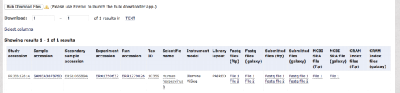
Click on Fastq file 1 under the heading Submitted files (ftp) this will download "Fastq file 1" to your PC/MAC download folder. Upload these fastq files to the Australian galaxy platform using the "GET DATA" function.
We cannot do anything until the item in the history on the right turns green so we wait … .
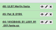
[keep on checking] Note: use your note book to keep a track of names as things will get confusing OR you can "edit" the data files using the pencil icon.
2) Map the NGS sequence data to UL97 using an alignment tool known as BOWTIE2
We are going to run BOWTIE2 via the galaxy platform (it will take a while)
In the end we will end up with 2 files for each sample we process: a .bam file with our data hidden in it and a .bai that helps other software arrange the data so we can visualise it.

a) The data you uploaded is not in the correct format for galaxy to use! You will need to ask the platform to first convert the data using FASTQ Groomer. The good thing is that galaxy has the option to run this process on multiple files automatically. In the picture above you will see the "one file" button shaded. Next to it is a "multi-file" button click on this and you can choose the multiple fastq data sets you have uploaded to the platform.
b) To use BOWTIE2 we will need our own reference genome. Return to the .fasta files you originally downloaded from NCBI. We will use the UL97_Merlin data which should be
named UL97_Merlin.fasta. This will be our 'reference' for BOWTIE2 so upload it to Galaxy using the Get Data function again.
[You will need to wait for this file to turn green before the next step]
You are now ready to activate BOWTIE2.
Note: If you have not already done so either use your note book to keep a track of names as things will get confusing OR you can "edit" the data file names using the pencil icon.
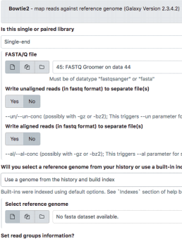
c) Once more we can do BOWTIE2 in a batch format by first clicking on the "multi-file" button (see image on left last page). Choose the Groomed data sets you wish to send through BOWTIE2 from the "FASTQ File" list. We now need to declare the genome source. Where it states "Will you select a reference genome…" Choose the "Use a genome from the history and build index" option. UL97_Merlin should come up automatically. Leave everything else as default and hit Execute.
d) Once everything goes green you can open the resulting files directly in to IGV via the link OR download the files and open them in IGV. This is all explained below in step 5.
3) Visualise the mapping results using the IGV software
Website:http://software.broadinstitute.org/software/igv/home
Method: Navigate to the IGV home using the above website and download the java
version of the IGV app. [This may cause some issues so will we may need to do some one-to-one troubleshooting]
Once open navigate to Genomes -> 'load genome from file' search your computer for the file UL97_Merlin.fasta you used for the BOWTIE2 step.
Navigate to File -> load from file and load the .bam files that correspond to the sample day you have chosen.
Navigate to Tracks -> fit data to window - this will fit all the data in the track window
What can you see? Open other .bam files that correspond to the sample days you have chosen. Can you see any differences? Hint: you can hide the coverage track.
Even at this point it is now worth reading through the paragraphs on the paper adjacent to the end of table 1. Can you see anything when comparing the paper to your visualisation of the data? Remember 1 codon = 3 base pairs or nucleotides
4) You will need to do this for UL54 as well!
Phase 3
1) Extract the consensus sequence from the BOWTIE2 alignments
We are almost there! If you hover over each .bam track in IGV and right click you get a popup menu list.
Chose copy consensus sequence from this list.
Go to your text editor and using copy/paste transfer just the DNA sequence to the list of sequences in the correct ULxx_ref.fasta file using the identifier “>Pat B [day]” .
Save the modified file as ULxx_ALL.fasta (where xx stands for 54 or 97).
2) Integrate the consensus sequences into the reference alignment and phylogenetic tree
Use the modified UL97_ALL.fasta file to repeat the alignment in step 3 with MEGAX. Tweek the nodes until the trees are the closest representation of Figure 3A/B
3) Compare our outputs to the description of UL54 and UL97 analysis in the paper.
4) You will also need to extract the percentage of each base called in the
identified codons - this data is required to reproduce aspects of figure 1
Now look at all your outputs in correlation to Houldcroft et al. Specifically compare the IGV visualization of the samples to the commentary and your equivalent of Figure 3A/B.
We will end the session with a group discussion of our experience in doing this exercise. I am sure there will be questions along the way. One question we will ask at the end will be “How can we integrate such analysis in to the clinic?”
2023-11-21
Use bioinformatics tools available on the internet to analyse data from Houldcroft et al.