Assignment 1 MATH 2028 2023 Final
Hello, dear friend, you can consult us at any time if you have any questions, add WeChat: daixieit
Note:
• All calculations in this assignment should be done by hand unless stated otherwise. Show your work.
• Include Matlab code and output whenever Matlab is required.
• All graphs should have title and axes labels.
1. This exercise is a typical final exam question (minus the Matlab content).
Consider the real signal below, periodic with period T = 4.

(a) What is ω0 for this signal?
(b) Use Matlab to graph this signal for −5 ≤ t ≤ 6.
(c) For which values of t will the Fourier series provide a good approximation for this signal? Use part (b) for justification.
(d) Use definition to find the complex Fourier coefficients cn. Consider special cases separately, if any. You may use an integration table with reference.
(e) Write the Matlab code to obtain the numerical values for c0, c1, c2 and c3, and compare to your answer in part (d).
(f) Find the real Fourier coefficients an and bn. You may use your findings from part (d).
(g) Find the exact value of the average energy of f(t) over a single period.
(h) Use Parseval’s identity and Matlab to determine how many terms, N, of the infinite complex Fourier Series are needed so that the approximation of the the signal with N terms retain at least 99% of the (average) energy of the signal f(t).
(i) Use Matlab to plot both the approximation and the signal f(t) on the same graph for −2 < t < 2.
(j) Draw a graph of the (complex) amplitude spectrum of f(t), containing at least the first 5 frequencies. Label angular frequencies present in this graph. You may draw the graph by hand or use Matlab or other suitable software.
[1+3+2+9+3+4+5+5+3+3=40 marks]
2. In this question, we use Matlab to do the computations.
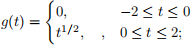
Consider the signal

(a) What is the (fundamental) period, T, for this signal?
(b) Plot the signal for 0 ≤ t ≤ T.
(c) Find the average energy of f(t).
(d) Obtain the complex Fourier coefficients c0, c1, c2, · · · , c5.
(e) Plot the approximation given by the

[4 × 5=20 marks]
3. This is a potential exam question on convolution.
Use integration to find the convolution of the two signals

[10 marks]
4. This is another convolution question, but it is to be done in Matlab .
Consider the following two signals f and g below, both are periodic with T = 4.
 (1)
(1)
and
 (2)
(2)
(a) Plot f ∗g for −4 ≤ t ≤ 4. Justify all your steps. (Note that I am not asking you to find the analytical formula for f ∗ g)

(b) Add commands to your the Matlab code that will request to input a value for t and show the value of f ∗ g(t) as an output. In other words, your code should be able to find a value of f ∗ g(t) for any value of t via input request.
[10 + 5 =15 marks]
5. This question is on the Geometry of Signals.
Consider the following signals over the interval −1 ≤ t ≤ 1.

(a) Show that f1, f2, f3 are orthogonal polynomial signals.
(b) Does {f1, f2, f3} form a basis for all polynomials of degree two or less? Give reasons.
(c) Find the next polynomial signal of degree 3 such, that they are all orthogonal.
[6+3+6=15 marks]
2023-11-18