Hello, dear friend, you can consult us at any time if you have any questions, add WeChat: daixieit

IEOR4742 – Deep Learning for OR & FE (Hirsa)

Problem Set

Problems 1 & 2 – Due date Oct 8, 2023 by midnight

Problem 1 (Impact of non-linear activation functions on Learning): One can show a feed-forward neural network with linear activation function and any number of hidden layers is equivalent to just a linear neural neural network with no hidden layer. Prove it.

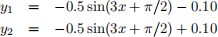
Problem 2 (Linear Classification Utilizing Hidden Layers): Assume Ω = [−1, 1] × [−1, 1]. Note this domain is an extended version of what discussed during the lecture. Define the following two curves in the two-dimensional space Ω

As described during the lecture, in linear classification we transform the space Ω using the following transformation to create new presentation for the space, that is for every grid point in Ω we do

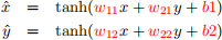
for some parameter set (w11, w12, w21, w22, b1, b2). One can run the following nested loop for the parameter set to visualize the transformed topology (sample code is provided for visualization purposes):

It is clear there are infinitely many presentations. We are looking for the one such that one can just draw a line

ax + by + c = 0

through the transformed data without crossing any of the transformed curves. Note that we seek w = (a, b, c) as well as (w11, w12, w21, w22, b1, b2) (9 parameters) to achieve this.

(a) use gradient-based (gradient descent) optimization routine to find the optimal parameter set (as explained in the sample codes)

(b) use various different starting points for the parameter set

(c) use different objective functions (e.g. hinge loss) in addition to the one that is provided in the lecture notes

(d) summarize your findings and observations and conclude

Problems 3, 4, & 5 – Due date Oct 21, 2023 by midnight

Problem 3 (Impact of different number of layers, different activation functions and optimization on learning): The code logistic regression multi 2layer.ipynb is a 2-layer logistic regression. The goal is to extend it to 3- & 4-layer logistic regression with different neurons and activation function for each layer utilizing different optimization routine to assess their impact on accuracy.

Consider the following six feedforward architectures:

(1) 1 st layer: tanh, 2nd layer: sigmoid, 3rd layer: leaky reLU

(2) 1 st layer: tanh, 2nd layer: sigmoid, 3rd layer: sigmoid, 4th layer: reLU

(3) 3 layers all sigmoid

(4) 3 layers all leaky reLU

(5) 4 layers all tanh

(6) 4 layers all leaky reLU

Try 50 & 100 neurons per layer and tf.train.RMSPropOptimizer.

Problem 4 (CIFAR-10): Repeat Problem 3 for CIFAR-10 dataset.

Problem 5 (visualization of the loss function): Use the first & second architecture and the optimization routine you were assigned in Problem 3 to assess the loss function by interpolation, namely the path traveled through the loss function from the starting point to the optimal point obtained by the optimizer (extension of example interpolation 2Layer.ipynb)

Problems 6 & 7 – Due date Nov 4, 2023 by midnight

Problem 6 (Convolutional Neural Networks): In the sample code example CNN MNIST.jpynb

(a) add one more convolutional layer with max pooling and assess the impact of extra convolutional layer on accuracy

(b) what are the number of parameters we are trying to learn in the original code and the new one with an extra layer?

Problem 7 (Batch Normalization): For Problem 6, assess the impact of batch normalization on learning (speed & accuracy)?

Problems 8 & 9 – Due date Nov 27, 2023 by midnight

Problem 8 (Generative Adversarial Networks - GANs): Rewrite the sample code example GANs.jpynb for the provided data (300 images) to train a GAN. You may use the snippets provided in exampleReadingSavingImages.ipyny to read and save images.

(a) use all images with random shuffling for training the GAN. For random shuffling you may use the below sample code (also provided in exampleReadingSavingImages.ipy

def next batch(data, batchSize):

#Return a total of ‘batchSize‘ random samples

idx = np.arange(0 , len(data))

np.random.shuffle(idx)

idx = idx[:batchSize]

data shuffle = array([data[i] for i in idx])

return data shuffle

(b) use 2 different autoencoders to create three different set of (300) images

(c) re-train the GAN using these 900 (300+600) images

(d) compare and assess your results in part (a) & (c)

Problem 9 (Deep Convolutional GAN): In building an architecture for a deep convolutional GAN, assume 5 convolutional layer for the generator using tf.layers.conv2d transpose and 5 covolutional layer for the discriminator using tf.layers.conv2d. Specify filters, kenrnel size, and strides in your architecture if your image sizes are 4096 × 4096.

Problem 10 – Due date Dec 6, 2023 by midnight

Problem 10 (Differentiable Neural Computers - DNCs): In the sample code DNC bAbI.ipynb for training the bAbI dataset we have used the following:

(a) memory matrix size 128 × 64

(b) number of read heads R = 4

(c) input size X = 159

(d) clipping gradient by value tf.clip by value in the range of 10

(e) number of iterations 10, 000

(f) optimizer tf.train.RMSPropOptimizer with learning rate of 0.001 and momentum 0.9

Assess the performance of the DNC architecture under different parameter sets and compare. Here are few scenarios:

(1) size of memory matrix 64 × 32

(2) number of read heads R = 3 or R = 5

(3) w/ & w/o gradient clipping by value tf.clip by value in the range of 6 & 8

(4) optimizer:

– tf.train.RMSPropOptimizer

– tf.train.AdamOptimizer

(5) number of iterations 20, 000

During testing for each scenario, do on both the original data and the manipulated data i.e. replacing the name of the object by it (e.g. replacing football by it in few places as discussed during the lecture).

Compare its performance with GPT 3.5 or GPT 4.0