ACS317 State Space Control Assignment
Hello, dear friend, you can consult us at any time if you have any questions, add WeChat: daixieit
ACS317 State Space Control Assignment
October 2023
Aims
1. To demonstrate how state-space control designs are carried out in practice.
2. To illustrate issues involved in controller and observer design.
3. To use MATLAB control systems toolbox commands and SIMULINK for the designs.
Objectives
At the end of the exercises, you will be able to:
1. Define a state-space model of a system.
2. Analyse the structural properties of linear systems using the state-space description.
3. Design a pole-placement state feedback controller for the regulator problem.
4. Design a feedforward gain to (almost) provide offset-free reference tracking to a step input.
5. Design integral control to achieve perfect offset-free reference tracking.
6. Design a state observer to estimate the states of the system.
7. Exploit the separation principle by combining the state feedback controller and state estimator into an output feedback controller.
8. Use MATLAB commands for offline system analysis and controller design.
9. Use SIMULINK to conveniently build and simulate the control system.
Note
MATLAB possesses well-written and extensive documentation that explainshow to use all of its in- built functions via the help and doc commands. For example, to obtain a brief description of the usage of the lqr command, simply type help lqr in the command window. For more extensive description, type doc lqr, instead. If you are unsure of what command to use for a particular task then make use of the search facility in the documentation. Remember, this documentation exists to help you, and should be your first point of call before seeking further help. Also, pay attention to any error messages that MATLAB throws out - they are actually very useful for trouble-shooting code.
Assessment and submission
This coursework constitutes 10% of your overall module mark and contains four exercises that are each worth 2.5% and are graded pass/fail. You will be supplied with a template MATLAB file (acs317.m) containing brief commented questions, to which you will provide brief commented an- swers. Once you have completed the exercises, you should submit your completed MATLAB file (acs317.m) and accompanying SIMULINK file (sslab.slx) to the coursework submission folder in Blackboard. Note - there is no lab report or anything else required other than those two files. The deadline to submit these files is 12 noon on Wednesday of week 12. This is an individual assign- ment - you may not collaborate with other students and instances of unfair means will be punished accordingly.
The System
The system under consideration is a chemical reactor shown in Figure 1. Note that this system has two inputs and three outputs. Typically the chemical reactor is regulated for disturbance rejection and to respond to step-wise commands for the reaction temperature and reactor pressure.
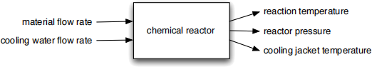
Figure 1: The chemical reactor system
By applying system identification techniques, a fourth-order model of the system is found, whose state space representation is given by

Here y1 is the reaction temperature, y2 is the reactor pressure, y3 is the cooling jacket temperature, u1 is the material flow rate and u2 is the cooling water flow rate.
The Laboratory
SIMULINK block diagram
You have been provided with a SIMULINK block diagram with filenamesslab.slx. This SIMULINK block diagram contains the chemical reactor system1. You will be modifying the block diagram to introduce controllers to the system. Also included in the SIMULINK block diagram is a partially constructed observer that you will connect to the system in Exercise 4.
MATLAB m-files
There are two m-files provided for this laboratory:
• The first m-file, named sslabsc.mis a set of initialisation instructions for the SIMULINK block diagram. It is important that you do not modify this file.
• The second m-file, name acs317.mis where you should write the code for the laboratory. Over the course of the laboratory, you will be addingto your commands, so you should make sure that you save this file at regular intervals.
Before You Start
You will be using MATLAB/SIMULINK. There are various ways to access this software - see https://www.sheffield.ac.uk/it-services/software/slmatlab
If installing the software, please make sure you include the Control Systems Toolbox in the installa- tion. Before you begin the laboratory you will need to follow these instructions:
1. Firstly, goto the ACS317 course folder in Blackboard. Then copy the files sslab.slx, sslabsc.m and acs317.m from the Coursework folder to a directory in your user area. For example, you
could create a folder in your U-drive called u:\lab and store the files in there.
2. Change MATLAB ’s working directory to the directory where you have stored the lab files. For example, to change to the u:\lab folder in MATLAB type
cd u:\lab
You will need to do this at the start of each session.
3. Type sslab to load the SIMULINK block diagram.
4. Type sslabsc to load the initialisation script.
5. Type edit acs317 to load the m-file ready for editing.
Exercise 1 - System Modelling and Analysis
1. Using the SIMULINK block diagram, investigate the open-loop step response of the chemical reactor system. To run a simulation, click on Start from the Simulation menu at the top of the SIMULINK window, and then inspect the relevant signals by double clicking on the scope blocks. Note that when SIMULINK runs a simulation of a continuous-time linear system, it is doing little more than computing the general solution of an LTI system, as you have studied in Lecture 7. For computational reasons, it must evaluate the general solution numerically and one way of doing this is by first computing an equivalent discrete-time system, as described in Lecture 8.
What can you infer about the system’s stability based on the response? Hint - does the magnitude of any of the responses grow in an unbounded fashion? Recall that system stability was covered in Lectures 5 and 6. Comment your answer in ACS317.m.
2. Using the model given on page 2 of this handout, form the system matrices A, B, C and D by adding the necessary commands to the acs317.m m-file. DO NOT USE THE SYSTEM MA- TRICES IN sslabsc.m. Use these matrices to define a state-space model of the system using the ss function. Add the necessary commands to your ACS317.m file to form the reachability and observability matrices using the MATLAB functions ctrband obsv.
Is the modelled system stable? Analysing the stability of systems in state-space form was covered in Lec- ture 6 and your finding should agree with part 1 above. Is the modelled system reachable and observable? These topics were covered in Lectures 10 and 11, respectively. Comment your answers in ACS317.m.
Exercise 2 - State Feedback and Feedforward Control
1. By choosing the desired eigenvalues to be −1 + 0.4i, − 1 − 0.4i, − 2 and −3, design a state feedback control gain matrix K using the pole placement method. With reference to Figure 2, introduce the necessary blocks and connections in the SIMULINK block diagram in order to ap- ply the feedback control to the system. To access the list of blocks, click on Library Browser from the View menu, or, alternatively, left-click in the SIMULINK window and begin typing the name of the block. Note that a state feedback controller can be implemented as a Gain block with multiplication defined for the matrix (K *u) case. Upon clicking on this block you will need to provide a gain. Rather than enter a matrix with numerical values, it is better to enter the name of the variable used in your .m file (e.g. ‘K’). This variable will be created in your workspace upon running the .m file, and SIMULINK will subsequently use this upon be- ing prompted to run a simulation. You will also need a Sum block for adding the reference inputs (set to zero in this instance through use of a Ground block) to the outputs from the state feedback gain, in order to provide the inputs to the plant. Pay close attention to the signs in the sum block or you could end up with positive feedback.
Simulate the response of the closed-loop system.
How does the closed-loop system response differ from the open loop case? How do the poles of the closed- loop system differ from those of the open-loop case? Recall that full state feedback by pole placement was covered in Lecture 12. Comment your answers in ACS317.m.
Optional: Once you have this working, feel free to play around with a different set of desired eigenvalues to see the effects on rise times, settling times, overshoots, etc.
2. The reactor pressure is to be controlled independently of the other two outputs. Design a feed- forward gain kr such that y1 +y3 andy2 have zero steady state error to the step reference signals. (Hint: define Cr in yr = Crx and then follow the steps from Lecture 14 in order compute kr, taking care with matrix dimensioning).
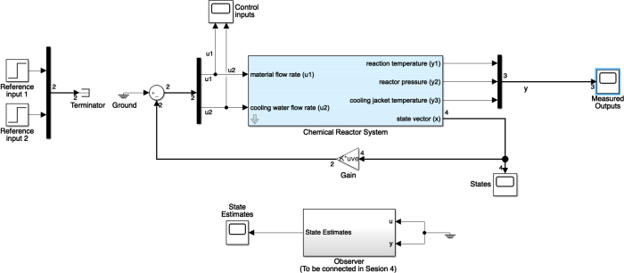
Figure 2: The chemical reactor system with full state feedback control.
Further hint regarding defining Cr:
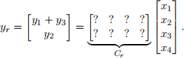
Use the relationships between y and x in equation (2) to determine the elements of Cr.
Further hint regarding defining feedforward matrices kx and ku used to form kr: pay attention to the dimension of the matrix on the right hand side of the following equation:
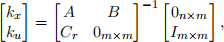
where 0n ×m is a n × m matrix of zeros, Im ×m is the m × m identity matrix, with n being the number of states and m being the number of control inputs, (which is equal to the number of controlled outputs, in this case). In order to extract kx and ku from the matrix on the left-hand- side of the above equation, you will need to use MATLAB array indexing2 commands.
By adding the necessary blocks and connections to the SIMULINK block diagram, according to Figure 3, introduce the feedforward controller to the system and investigate the step response of the closed loop system. Check the design by comparing the reference outputs to the reference inputs (as viewable in the Scope block in the top right of Figure 3).
Do the reference outputs perfectly track the step inputs at steady state? Hint - are your modelled system matrices (1), (2) the same as the ones used in the simulation model? (The latter can be found in the sslabsc.m file). Comment your answer in ACS317.m.

Figure 3: The chemical reactor system with full state feedback control and feedforward control for reference tracking.
Exercise 3 - Optimal Control and Integral Control
1. By adding the appropriate commands to your m-file, design an infinite horizon linear quadratic optimal regulator (studied in Lecture 13) with the following design matrices:
Qx = C’ * C
Qu = rho * eye(2)
and choose rho=1. This particular choice of state penalty matrix Qx penalises non-zero values
of those states that form the measured outputs of the system.
What are the closed-loop system eigenvalues?
Optional: Play around with different values of rho to see the effect that penalising the controls has on the output responses. Also, feel free to try arbitrary choices for Qx and Qu.
2. Following the procedure in Exercise 2, Question 2, design kr for zero steady state error using the new controller and investigate the step response of the system.
Are the transient and steady-state responses qualitatively different from those obtained using pole- placement state feedback control design? Comment your answer in ACS317.m.
3. In order to achieve offset-free reference tracking, you will now include integral action in your controller, and will design this through an LQR approach. Firstly, let’s define a new cost func- tion to reflect the fact that we have augmented the state vector with two new additional states that describe the integral of the difference between the reference inputs and reference outputs:

Note that the upper left 4 × 4 sub-matrix of Qx contains the same state penalty terms as used in part 1 (C’ * C), whilst the bottom right 2 × 2 sub-matrix contains the weights w1 and w2 that penalisethe new states associated with integral action. Set w1 = w2 = 10 to define the new state penalty matrix. Then use the same approach as in part 1 to design a LQR controller for the augmented system (see Lecture 15 notes).
Check that the closed-loop system is stable by inspecting the eigenvalues of the closed-loop augmented dynamics matrix.
4. Modify the SIMULINK block diagram to incorporate the integral action and necessary feedback connections, as shown in Figure 4. Hint - the LQR controller from part 3 is of the form Kaug = lK −ki]. You will therefore have to extract K and ki from Kaug, so you need to know the dimensions of both matrices. These are as follows: K ∈ Rm ×n, ki ∈ Rm ×q, where q is the number of controlled outputs (which is equal to the number of control inputs m, in this case). Also bear in mind that the state feedback controller K maybe different to that from part 1, and so it’s good practice to re-synthesise the feedforward controller kr using the same method as in part 2.
Investigate the step response of the system. What is the steady state error between the reference inputs and reference outputs? Comment your answer in ACS317.m.
Optional: Investigate the effect on settling time and overshoot of choosing different weights w1 and w2 .

Figure 4: The chemical reactor system with full state feedback + integral control and feedforward control for reference tracking. Note the 1/s Integrator block.
Exercise 4 - Observer Design and Output Feedback Control
1. By choosing the desired eigenvalues to be to be −2 + 0.4i, − 2 − 0.4i, − 4 and −6, design a full-state observer gain matrix L using the pole placement method. Recall that observer design by pole placement was studied in Lecture 16.
Check that the error dynamics are stable.
2. By modifying the SIMULINK block diagram, connect the observer block according to Figure 5. Double-click on the observer block and build the connections as drawn in slide 6 of Lecture 16 notes (the matrices are all implemented as Gain blocks. You’ll also need an Integrator block - use the default initial condition of 0 in this). Recall that an observer is a system, and so has inputs (control signals u and measurements y) and outputs (state estimates ˆ(x)). Then run a
simulation and compare the graphed responses of the state estimates to the actual states.
Do the the state estimates from the observer closely match the actual states? Comment your answer in ACS317.m
Optional: Investigate the design with a different set of desired observer eigenvalues and ob- serve the error dynamics. Also try different initial conditions on the states of the observer (set via the initial condition of the Integrator block within the observer). You may also wish to design the observer gain matrix using the kalman command.
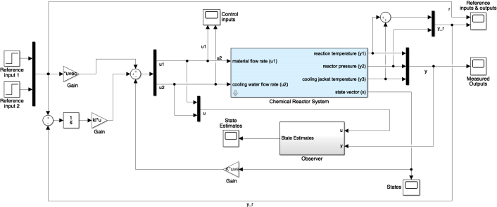
Figure 5: The chemical reactor system with the observer partially plumbed in.
3. Finally, form an output feedback controller by feeding the state estimates from the observer into the state-feedback controller, according to Figure 6. Simulate this final closed-loop system. Do you still achieve steady-state offset-free reference tracking with your output feedback controller? Comment your answer in ACS317.m
If everything has gone well, you closed-loop simulated responses should look similar to those in Figure 7. If so, then submit your work. When marking your work, I will run your ACS317.m script, and then perform a simulation using your final sslab.slx file. If your responses are qualitatively similar to those in the figure (i.e. achieve steady-state offset-free reference track- ing in response to the step reference inputs), and the majority of your commented answers in ACS317.m are correct, then you will be awarded the full 10% for this coursework.

Figure 6: The chemical reactor system with the observer fully plumbed into provide output feedback control.

Figure 7: Example of closed-loop responses with output feedback control, showing the controlled outputsyr (red, green) tracking the step reference inputs r (yellow, blue).
Summary
In the process of carrying out these exercises, you will have learned to use the MATLAB control systems toolbox commands relevant to state-space design methods and used the SIMULINK environ-ment to implement the designs and evaluate the system responses. You will also have developed an appreciation of the effect your design choices have on the system responses. The questions at the end of each of the steps in the exercises were to reinforce the relevant concepts through the various designs and observations of system responses.
2023-11-10