Hello, dear friend, you can consult us at any time if you have any questions, add WeChat: daixieit

Economics 443

Labor Economics

Autumn 2023

Homework 5

Labor Demand

Stata

Be clear in your solutions when lines and curves are tangent and when they aren’t. 

1. Suppose the hourly wage is $10 and the price of each unit of capital is $25. The price of output is constant at $50 per unit. The production function is

f(E,K) = E^½K ^½,

so that the marginal product of labor is:

MP_E = (½)(K/E) ^½ .

If the current capital stock is fixed at 1,600 units, how much labor should the firm employ in the short run?  How much profit will the firm earn?

2.  Megatech assembles calculators using labor (E) and robots (K).  Megatech earns $ 72 for each calculator it sells.  Labor (E) costs $9 per hour.  Each robot is valued at $12.32 per hour.  Megatech has 27 robots and cannot buy or sell robots.    Megatech’s production function is:

  q = f(E,K) = 64E^1/3K^1/3

a. What is the expression for Megatech’s marginal product of labor? 

b. What is the expression for Megatech’s value of marginal product of labor?

c.  How many hours of labor will Megatech employ to maximize profits?    

d. What is the marginal product of labor when Megatech maximimizes profits?

e. What is the value of marginal product of labor when Megatech maximizes profits?

3.   Colorado Inc. is an e-tailer that processes orders with labor and capital.  Colorado must process 300 orders this month.  Labor costs $10 per hour and capital costs $30 per hour.  Colorado’s production function is:  

q = f(E, K) = EK

where q is number of orders processed, E is the number of hour of labor and K is the units of capital stock.

Elaina:   This is only long run.

a. How much labor and capital will Colorado employ to minimize the total cost of processing 300 orders in the long run?  What is Colorado’s total cost to process these orders? 

3.   Data for this problem are in the file Econ443_HW7_PSID that’s posted on Canvas.  The columns are the variables:

unqid: id code for the subject

hours:   annual hours of work

wagert:   hourly wage rate

yrsed:   years of education

white:   subject is white

age:  age of subject.

a.   Transfer the data to Stata and save the data in a Stata .dta file.

b.   Write a program that summarizes the data and runs the following regressions:

hours = α + βwagert + ε

wagert = α + βyrsed + γwhite + ε

c.  Interpret the first regression in one sentence.   What is the implied labor supply elasticity?

d.  Interpret the second regression in a short paragraph.

4.  BLS data in Stata

a.  Retrieve the following series of data for the period January 1948 to September 2023 to September on separate graphs.  Data are from Table 1 of CPS Historical Data.   All should be seasonally adjusted.

(a) Unemployment rate of women age 20-plus

(b) Unemployment rate of men age 20-plus

(c) Unemployment rate, both sexes, age 16-19 

Data are from Table 1 of CPS Historical Data.   All data should be seasonally adjusted.   You have done up to this step for HW4. 

(i.) Download the Excel files, edit the excel files so you have a single file that can be readily transferred to Stata.

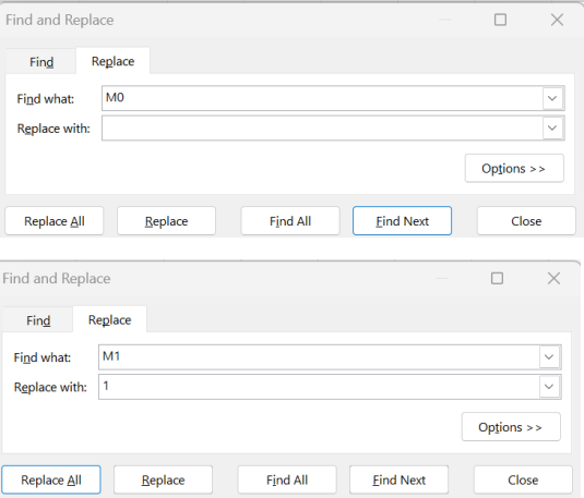
You will have to make sure that the series are aligned.   You will need to change the “period” variable (which is month) so there is no “M” in front with the following commands in excel and selecting “Replace All”.  (This will allow Stata to read the variable in as a number rather than a character.)

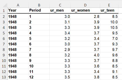
The first 13 lines of the Stata file will be.

(ii.)  Transfer the data into Stata.   In Excel, select the variable names and all the data.   This will be 910 rows and 5 columns.   Select “copy”.   Go into Stata and select “Data”, “Data Editor”, “Edit”.   Paste the data into the top left cell.   

For some reason, the copy/paste doesn’t always work the first time (for me) so you may also need to repeat this step.

Stata will ask you whether to transfer the first row as variable names or data.  Select “variable names.”

Save the data.

 (iii.) Write a .do file that graphs the three series over time.   The following two commands should be in your .do file.   

generate time = year + (period – 1)/12

generate difference = ur_men – ur_women

Graph the three unemployment rate variables over time.

Graph “difference” against time.

Submitting your solutions to Questions 3 and 4.    Copy and paste your .log file and any graphs into a Word file.  Convert the Word file to .pdf and submit the .pdf.  Your .do file and .log file names should include your name.   The title of the graph should include your name.

The document Econ443_Au23_Lecture8_Stata_21Oct23 has a template for a .do file.   There is a tutorial that goes through the document posted onCanvas.