CIVE4095 short and long term wave analysis Coursework
Hello, dear friend, you can consult us at any time if you have any questions, add WeChat: daixieit
CIVE4095
Department of Civil Engineering
Coursework 1: short and long term wave analysis Coursework
1 Objective of Coursework 1
Using the data provided for the Poole Bay (UK) wave measurement buoy (see Fig. 1 for the position of the buoy), compute the main statistical parameters that describe an individual sea state that was mea- sured (short term wave analysis) and the parameters that describe the wave climate and the probability of occurrence of extreme sea states (long term wave analysis).
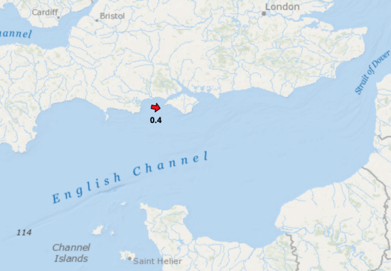
Figure 1: Position of the Poole Bay Waverider buoy (http://wavenet.cefas.co.uk/Map retrieved 06/07/2022)
2 Data
The data provided were measured between 2013 and 2019 by the Waverider buoy located in Poole Bay (Latitude: 50.633333 N Longitude: 1.721111 W) and managed by the Cefas (Centre for Environment, Fisheries and Aquaculture Science). Four types of data files are provided and available for download on Moodle. The physical constants to be used in the coursework are g = 9.81 m/s2 (g being the gravity acceleration) and ρ = 1025 kg/m3 (ρ being the density of water).
. Time series.xlsx: this file contains the time series of the free surface during a sea state recorded by the buoy. The file has two columns, which contain: time (in seconds) in the first column, and free surface elevation (in metres) in the second column. The free surface elevation is relative to the mean water depth during the interval of measurement.
. Energy density spectrum.xlsx: this file contains the energy density spectrum of the same sea state of the file Time series.xlsx. The file has two columns: frequency (in Hz) in the first column and spectral energy density (in m2 /Hz) in the second column.
. cleaned data poole bay.xlsx

 containing a table with the main parameters of all the sea states recorded by the buoy between 2013 and 2019 every half an hour. Although data that were clearly not valid were removed, spikes in the direction of propagation are present, however consider these data valid and include them in the analysis. The first row in the spreadsheet indicates the parameters in each column. Note that missing data are identified with a code 9999. The significant wave height (Hs), main direction of propagation (θm) and mean wave period Tz are shown in Fig. 2.

Figure 2: Hs , θm, and Tz measured by the Poole Bay waverider buoy between 2013-2019
. Table ![]() sea states poole.xlsx contains a table with the number of sea states that occurred
sea states poole.xlsx contains a table with the number of sea states that occurred![]()
![]()
in each bin identified by an interval of in significant wave height (Hs) and main direction of
propagation (θm), during the whole period of measurements (2013-19). The first two rows of the spreadsheet indicate the intervals in Hs chosen and the first column indicates the intervals in θm chosen. The number in each cell is the number of sea states on record that fall into the bin specified by the considered interval in Hs and in θm. Note that while intervals in θm are uniform
(every 10 degrees), the intervals in Hs are not. The reason for that is explained in class.
3 Coursework tasks
Coursework tasks are here listed. The marks assigned to each task are indicated in square brackets.
. For the measured sea state provided in the file Time ![]() series.xlsx compute Hs, and the mean period Tz, using both the zero up-crossing analysis and the spectral analysis (the spectral density of energy is provided in the file Energy density spectrum.xlsx)
series.xlsx compute Hs, and the mean period Tz, using both the zero up-crossing analysis and the spectral analysis (the spectral density of energy is provided in the file Energy density spectrum.xlsx)
 . Discuss the differences for the results of Hs, and Tz obtained with the two methods. Also, compute the power per unit
wave front Pref for the sea state under study. [15/100]
. For thesea state provided in the file Time series.xls, assuming that individual waves follow the Rayleigh distribution, compute Hrms and the wave height that has probability of not being exceeded equal to 0.93. Plot the Rayleigh cumulative distribution curve and identify on the graph
Hs and H1/10. [15/100]
. Compute the probability of occurrence of sea states as a function of Hs and θm, using the intervals of Hs and θm used in the provided table (see Table ![]() sea states poole.xlsx)
sea states poole.xlsx)![]()
![]() . Describe the wave climate in Poole Bay by identifying the sectors of propagation of the waves and by computing the omni-directional cumulative probability for the sea states. Identify the Hs that is not exceeded by either the 98% or 99% (as you prefer) of the sea states on record (this is the
. Describe the wave climate in Poole Bay by identifying the sectors of propagation of the waves and by computing the omni-directional cumulative probability for the sea states. Identify the Hs that is not exceeded by either the 98% or 99% (as you prefer) of the sea states on record (this is the
value will be used as threshold for the Peak Over Threshold, POT, analysis). [20/100]
. Compute, using the POT method, the values of Hs with return period of 1, 5 and 60 years using the Gumbel distribution. Discuss the results, with focus on the fit of the data to the theoretical distribution. [25/100]
. Summarise the results and the methodology followed in a report of no more than 2000 words
(excluding figure captions, formulas, and references). [10/100]
. Optional: compute, using the POT method and another extreme value distribution (for example the Weibull distribution explained in this document), the values of Hs with return period of 10, 50
and 100 years. Compare the results with those obtained using the Gumbel distribution. [15/100]
4 Further extreme value distributions.
The Gumbel distribution is part of a family of three extreme value distributions commonly used in engineering. The other two are the Fr´echet and the Weibull distribution. Usually, for a given series of extreme values, the parameters of more than one distribution are computed and the fit to the distributions is compared to select the best fitting one. Alternatively, the Generalised Extreme Value (GEV) distribution can be used; this distribution combines all three aforementioned
distributions (see Coles, 2001 Section 3.1.3).
Here the Weibull cumulative distribution is examined. This is written as:
 (1)
(1)
λ ≥ 0 being the location parameter, and β > 0 being the shape parameter. These two parameters need to be computed using the Method of Moments (MoM), however this is not as simple as in the case of the Gumbel distribution. The mean and the variance of the distribution, assumed to
be equal to the samples ones, are:
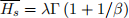 (2)
(2)
and:
 (3)
(3)
Where Γ is the gamma function (Excel and MATLAB both compute gamma function with a
built-in function). The coefficient of variation V , i.e. the ratio of the standard deviation (s) to![]()
the mean (Hs) of Hs, i.e. V = s/Hs, is:
 (4)
(4)
If Hs and s are known the values of the parameters λ and β can be determined by solving Eq.
(4) with β as the unknown, using numerical iteration. Then λ can be estimated using Eq. (2),
i.e.:
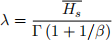 (5)
(5)
As done for the Gumbel distribution it is convenient to plot the distribution on a probability chart, i.e. a system of coordinates in which the distribution appears as a straight line. For the Weibull
distribution:
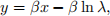 (6)
(6)
where:
 (7)
(7)
and
 (8)
(8)
The test-fit to the distribution is done as for the Gumbel distribution, i.e. following Step 3 with the values for y and x computed for the samples. The Frechet distribution has also two parameters and can be determined as well the MoM. The reader is referred to Kottegoda and Rosso (2008)
(Section 7.2.2 to 7.2.4), available at the Green’s library, for the relationships.
5 Tips for the coursework
Submission
Submission deadline is November 10th 2022 at 15:00 on MOODLE only. Note that you will have to submit the report in a single pdf file and confirm the submission, otherwise it will stay
as a draft.
Handling the large data file to find storms over threshold
In order to find the peaks of the storms over the Hs threshold from the file provided you have to identify these storms in the data and then select the peak Hs for each storm. There are many ways to do that; here I will give you some tips for working in Excel. The first option to select maxima is to filter data using the ”Filter Data” function in Excel (see Fig. 3), you want to retain
data for which Hs is larger than the threshold value and smaller than 9999.

Figure 3: Excel ”Filter Data” options to select the storms with Hs larger than the threshold.
Once you assign this filter only the rows that satisfy the two conditions will appear. If you prefer to retain all the rows, one quick way to visualise Hs over threshold is to use conditional formatting by highlighting in, for example, red the cells with values of Hs exceeding the threshold (see Fig.
4). Pay attention to the missing data code (9999), it is suggested to replace these values with
blank cells so the code cannot interfere with highlighting cells and plots. To do so you can use the function find and replace in Excel (CTRL+F) (see Fig. 5).
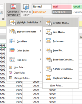
Figure 4: Excel ”Conditional Formatting” options to highlight the cells with Hs larger than the threshold.

Figure 5: Example find and replace function to remove 9999 codes.
Selecting peaks using the POT method
When selecting peaks keep in mind the restrictive conditions that have been introduced in the notes and in the worked example. If you have any doubt about retaining or removing data, make a decision based on the information in the notes. Take a consistent approach and, above all, justify
your choices in the report.
Structure of the report
Technical and scientific reports have a pretty standard structure, which you should follow in this coursework. Start with an Introduction section to explain the background and objectives of your analysis: which location are you studying? Which data? What are the parameters that you have to compute? The introduction does not need to be long, but it should give an idea of the background of your study in few sentences. The next section is the Methodology. For each of the objectives in the brief show how you compute the required parameters, introduce the equations and variables involved. Label each equation and introduce each variable used. Next is the Results, or Results and discussion, section. This shows the results and discusses it (Discussion can be a separate or joined section). Finally a Conclusion section rounds up the document. Although here this section is not very important, pay attention to avoid to use it as a summary. This section should answer to the questions: have you achieved your objectives and to which extent? Are there limitations in your work, which ones? What needs to be done next?
DOs and DON’Ts
– The report must be prepared INDIVIDUALLY in all its parts.
– Be CONCISE and to the point. Prioritise quality over quantity.
– DO present the location and data in the introduction. You need to make the report accessible to a reader who does not know anything about the location studied.
– DO state which equations and parameters have been used, focus on the results and analysis of them.
– DO provide details of the computations done, but if they consists in large tables include them in an Appendix.
– DO describe and analyse each table or plot introduced, DO NOT include a graph or a table that is not explained in the text.
– DO avoid bullet points.
– DO consider the number of decimal places when presenting numbers (as opposed to using them in calculations), e.g. Hs should be expressed with 2 decimal places.
– DO NOT include in the text parts of or whole scripts used for the coursework (for example in Excel or MATLAB). DO NOT describe what done with the software used, focus on the general methodology.
6 References
Kottegoda, N.T. and Rosso, R., 2008. Applied statistics for civil and environmental engineers (p.
718). Malden, MA: Blackwell.
Coles, S., 2001. An introduction to statistical modeling of extreme values (Vol. 208, p. 208).
London: Springer.
2023-11-09