The objective is to study a) application of copulas to risk factor modeling and b) options portfolio VaR.

File: assign3-templ.xlsx

Video: “Assignment 3 Video Companion” on YT

Introduction

Your task is to quantify market risk exposure of the customer’s equity index options portfolio. The workflow:

1.    Map the portfolio to its risk factors

2.    Analyze the risk factors, then generate hypothetical scenarios of risk factors

3.    Apply option pricing to the portfolio securities under the generated scenarios to obtain market values of portfolios

4.    Calculate the 99% value at risk by obtaining the 99th  quantile of the profit and loss distribution of the portfolio under the scenarios

The final answer of this assignment is the portfolio 99% VaR.

Portfolio

The portfolio positions are given in Sheet “Portfolio” as shown below. Note the current market value of the

portfolio under “Total” column. Study the Excel equation in the cell to understand how to calculate the

portfolio market value (MV)  given the prices p!  of securities and their holdings h!   because you will need this in simulation step:

Note, that this portfolio implements the Front Spread strategy with the following payoff profile:

Note, that the upside is limited and reaches maximum when the stock price is equal to the strike price of the short options, in our case it is 2790. Also, note that the downside is potentially unlimited since the

underlying price is potentially unlimited. In practical terms it means that the losses can be very large.

Therefore, special attention needs to be paid to this type of strategies: they can lead to large losses to the broker, not only the client.

Black Scholes, 2 points

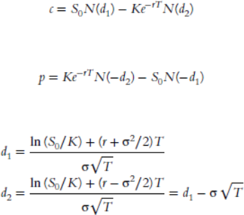
The option portfolio is on SPX underlying, which is an index. The index doesn’t pay dividends, and options are European. Therefore, you can use the equation from the textbook or the slides in Week 4:

All the relevant inputs are in the portfolio security details. I copied them from Bloomberg terminal below. Though you don’t need to extract data from Bloomberg screenshot yourself, I already did it for you.

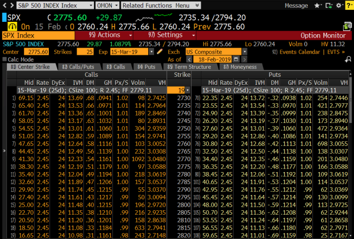
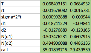
You have to implement the Black Scholes equations in cells B14:C21 replacing my pre-calculated numbers, and if you do it right the numbers should match mine:

Mapping Risk Factors to Portfolio, 2 points

Our portfolio has two options with underlying SPX index. The options are expiring in 25 days. Therefore, we can map this portfolio to two risk factors: SPX Index and VIX index. The former is obvious it’sthe option

underlying price. The latter is the volatility index, seehttp://www.cboe.com/vix. It’s calculated from implied volatilities on options expiring about a month forward.

I downloaded the historical series of SPX and VIX in “idx” sheet. You have to calculate the continuous returns of two indices in columns D and H:

The numbers should match my numbers, which you should replace with your equations.

Scenario Generation with Copulas, 3 points

1 point

Once we obtained the historical series, in order to apply copulas we need to estimate the marginal and

copula parameters. For this exercise we’re going to assume that the marginal distributions are Normal. The   simplest estimation of marginal distribution is by obtaining the sample mean and the variance. We are using only year 2006 in this estimation. I calculated them for SPX in cells F2:F3 of sheet “OPTN Port Copula.” You    should do the same for VIX distribution parameters in cells F4:F5.

In this exercise we’re going to use Gaussian copula and use the sample correlation as its parameter p. This is not how it’s done in real application, but it’s too much work for you to implement the copula fitting in Excel. So, we’re skipping this step.

Once we have marginal and the copula, we can use them to generate risk factor scenarios. We’ll generate 1,000 scenarios. First, we generate the independent uniform random numbers in columns B and C. Use

Excel RAND() function, and replace the prepopulated cells with your equations.

Now we need to plug these random numbers into copula, and get the new set of correlated uniform random numbers. I did it for you in columns H and I:

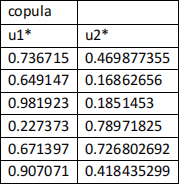
Analyze the formulas, and continue them to the remaining simulations in these columns replacing cells in green.

2 points

Final step is convert the uniform random numbers into risk factors by applying the corresponding inverse marginal distributions. Analyze the equation in column J to see how it’s done for SPX. Continue the

equations to all simulations replacing green cells in column J. The idea is that we model the risk factor as

N(, S %) where   is the sample mean and S%  is the sample variance. We can use inverse CDF in Excel

NORM.INV(x,mean,stdev) to get the inverse marginal distribution.

Now, apply the same logic to obtain VIX returns in columns K using appropriate parameters.

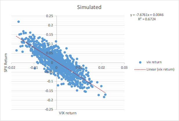
If you did everything right, then you should get a scatter plot of 1,000 simulated scenarios similar to the one below:

Portfolio Market Value Simulation, 1 Points

Next step is calculate the scenario option values in columns P and Q for a long and short call options. You have to implement Black Scholes equations. I suggest to use columns R:AG for intermediate calculations.  Use the equations that you implemented in Portfolio sheet.

In this step you have to generate the stock price and volatility under the scenarios that we generated in the previous step. Remember that columns J:K contain the SPX and VIX returns for each scenario. Use these

values to obtain scenario price and volatility by inverting the return equation:

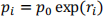
The initial value of price and volatility are those in the “Portfolio” sheet. For instance, in the following

example shown in the figure I applied the scenario return on vix -0.016144 to the initial value of long call volatility 12.04% to get the scenario volatility 11.85%.

Portfolio VaR, 2 points

Once you got the option prices under 1,000 scenarios, you must calculate the portfolio value in column AI. The equation is similar to the one used in Portfolio sheet. Profits and Losses as well as the returns are pre- calculated for you in columns AJ:AK.

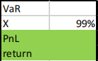
The final step is calculate VaR in dollars and as a return. You have to implement the equations in cells AN3:AN4.

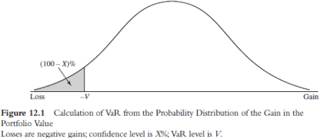
The idea is to use Excel PERCENTILE() function. You have to understand how it can be used to obtain VaR as a tail of profit and loss distribution. We discussed it the class several times, see also the figure from Week 4 class below. You’re looking for a value “V.”

For your reference my values were as follows.

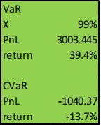
Your values will be different, but should not be too different. This is the main result of this exercise.

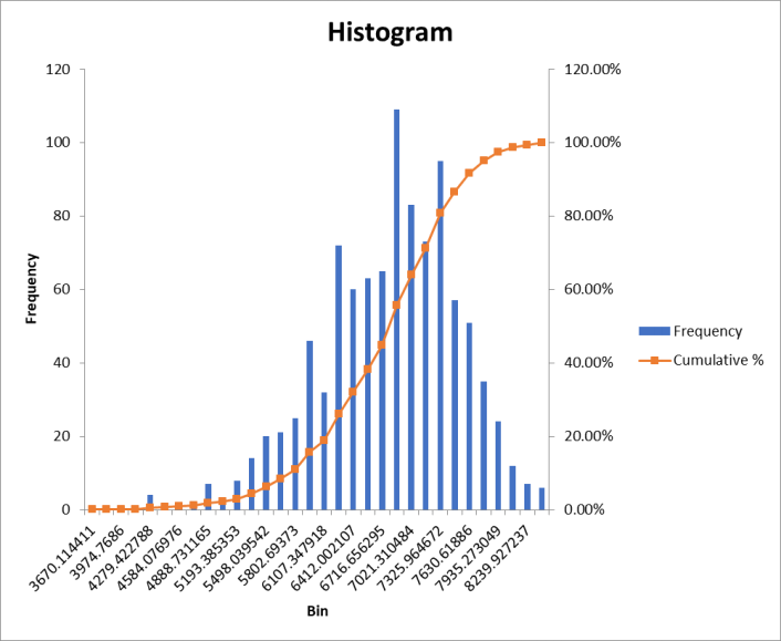
Produce the histogram of the portfolio market values in column AI. Use Excel’s “Data Analysis” add-in and   put the histogram in a separate sheet “ Port MV Hist” . My histogram looked as follows, and yours should be similar:

CVaR

Conditional VaR is the average loss larger than the VaR. It is discussed in the textbook. I implemented an equation for CVaR in cells AN8:AN9, please, study them.