Hello, dear friend, you can consult us at any time if you have any questions, add WeChat: daixieit

EC 205: MACROECONOMIC THEORY I

FALL 2021

HOMEWORK 1

1 Business Cycle Statistics and Stylized Facts (2 Points)

In this first part, you will learn how to produce business cycle statistics similar to those we saw in lecture. More specifically, you will need to obtain the following time series for the U.S. for the period spanning 1990Q1 to 2019Q4: nominal private consumption, nominal fixed private investment (a measure of physical capital investment), nominal Gross Domestic Product (GDP), the GDP deflator, and the consumer price index (CPI). The Saint Louis Fed’s FRED database is an excellent source that compiles different databases, but you may use other sources if you prefer as long as the series you use are the correct ones. In what follows, you must clearly specify the source of the series you use. Using the time series above, do the following:

1. (0.5 Points) Using the GDP deflator, generate the real series for all relevant variables. Separately, create a measure of gross consumer price inflation using the CPI.

2. (0.5 Points) Following the procedure we saw in lecture for the variables you created in 1.—that is, taking natural logs, etc. . .—use the Hodrick-Prescott (HP) filter with smoothing parameter 1600 to obtain the cyclical component of these series, and plot the cyclical series you obtain in a single graph. The figures must be legible, with clear legends/axes. The figures must also include a footnote specifying the data sources and any other information you deem relevant so that the figure is self-contained. You can use Stata’s HP filter or, alternatively, Matlab’s. For details on how to use the HP filter in Matlab, see: http://www.mathworks.com/help/econ/hpfilter.html.

3. (1 Point) Compute the standard deviation, contemporaneous correlation, and first-order autocorrela-tion of each of the cyclical series you obtained in 2. Clearly document these second moments in a table similar to the one we saw in lecture

2 The Prototypical RBC Model with Taxes (8 Points)

Consider a decentralized-economy RBC model with distortionary taxation. All markets are perfectly com-petitive. Specifically, assume that the government (a passive agent in this economy) collects revenue using both lump-sum taxes and proportional consumption, labor income, payroll, capital accumulation, and profit taxes. Revenue from taxation is used to finance an exogenous government spending stream given by (in other words, follows an exogenous process, very much like TFP ) as well as a subsidy on capital purchases by firms. These taxes (and tax rates) are denoted by and respectively (the proportional taxes take values between 0 and 1, are taken as given, and are exogenous). The subsidy rate on capital purchases is . Assume that the household accumulates capital. First, you will work with general functional forms. I will then ask you to use specific functional forms and express the equilibrium conditions of the model using the latter.

2.1 The Household’s Problem (2.75 Points)

The household’s problem is to

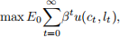
subject to

and the time constraint

for given, where denotes labor supply, is leisure, denotes capital supply, and the household has a time endowment of 1 unit. Utility is increasing and concave in each of its arguments. denotes the real wage, is the real return on capital, is the household’s subjective discount factor and is the depreciation rate of capital. are lump-sum firm profits, which the household takes as given. Answer the following questions:

1. (0.25 Points) What are the state (separated into two categories, exogenous and endogenous) and control variables?

2. (0.25 Points) What happens to the budget constraint if all tax rates (except lump-sum taxes) are 0 for all t?

3. (1 Point) State the law of motion for capital (that is, characterize how investment is given in this model).

4. (0.25 Points) Write down the household’s Lagrangian, find the first-order conditions, and characterize the household’s optimality conditions.

5. (0.25 Points) Explicitly describe the economic intuition behind each of the optimality conditions you obtained in 4. as we have done in class.

6. (0.25 Points) Assume that the utility function is given by where is the relative risk aversion parameter, captures the weight that we assign to the disutility from working, and is the parameter that dictates the elasticity of labor supply. Rewrite the conditions you found in 5. using this specific functional form.

7. (0.5 Points) Imposing steady state, formally analyze the effect of an increase in on labor supply.

2.2 The Firm’s Problem (2.25 Points)

The firm’s problem is very simple. Firms maximize profits inclusive of profit taxes, which are given by

where is exogenous aggregate productivity, is a standard constant-returns-to-scale production function, increasing in both arguments, is a proportional payroll tax, are profits taxes, and is the capital purchases subsidy rate (all proportional taxes/subsidies take values between 0 and 1 and are taken as given by firms). Answer the following questions:

1. (0.25 Points) Find the optimal demand for labor

2. (0.25 Points) Find the optimal demand for capital

3. (0.75 Points) Assuming that where is the capital share, write down the conditions in 1. and 2. using this functional form. How is capital demand affected by an increase in ?

4. (0.25 Points) What effects do profits taxes have on firms’ optimal input-demand decisions? Explain the intuition behind your findings.

5. (0.75 Points) Now, go back to the optimal capital accumulation decision you obtained in the household’s problem in 2.1.4 and plug in the optimal demand for capital you obtained in 2.2.2. Imposing steady state on the condition you obtain, formally analyze how an increase in affects the optimal amount of capital.

2.3 The Government (1.5 Points)

We have not explicitly seen a model that introduces government spending in class. Write down the gov-ernment’s budget constraint assuming that government spending is exogenous (Think intuitively about the sources of revenue for the government using the household’s budget constraint and the firm’s problem, assuming market clearing in all markets).

2.4 Closing the Model (1.5 Points)

Answer the following questions:

1. (1 Point) Using the household’s budget constraint, the firm’s problem. and the government budget constraint, impose market clearing (that is, supply is equal to demand in all markets) and derive the economy’s resource constraint. Explicitly show the steps you follow to obtain this constraint.

2. (0.5 Points) Define the equilibrium of the economy as we did in lecture (”Taking the exogenous processes as given, the allocations {...} and prices {...} satisfy...”) (Make sure you have the same number of equations as unknowns!)