This tutorial is reviewing some questions which cover topics in week 6 to week 12.

1.1    Series

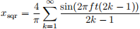
Digital electronics are used to produce discrete signals.  One such signal that has wide application is the square wave. A square wave is a non-sinusoidal periodic waveform that alternates at a constant frequency between fixed minimum and maximum values, with the same duration at minimum and maximum. They are often used in conjunction with analogue circuits to produce continuous signals, e.g. for sound synthesis.  For this reason, it is very useful to have a them in symbolic form.  A  Fourier series can  be used to represent any periodic function as a summation of cosines and sines. A square wave may be expressed as the following Fourier series expansion:

To do this in MATLAB, we express the series as a sum of symbolic terms.  This requires the use of the symsum function.  Its help function is given below:

Write a MATLAB code to construct and plot a square wave by Fourier series expansion using symsum.

1.2    Newton Raphson’s Method

Suppose we wish to find the zeros of a function, but cannot compute its derivative everywhere.

For example, this problem might arise if the absolute value function f (x) = |x|  is employed, because the function cannot be differentiated at 0.  Or at the far extreme, the function itself may not be differentiable anywhere, such as the Weierstrass function:

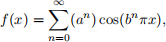
where 0 < a < 1, b is a positive odd integer, and ab > 1 + 3/2π.

In these cases, Newton’s method fails, as it relies on an expression for the partial derivatives (Jacobian). So the question is:  How do you do gradient descent without a gradient?

1.3    Differential Equations

This example shows the recommended way to assess the output of a variable-step solver such as ode45 for first-order odes. Supplying a time vector instead of a time span to the solver ensures the returned reference and student solutions are evaluated at the same time points without forcing a specific approach.

The Lotka-Volterra predator-prey model uses first-order differential equations to estimate the populations of two interacting species, p1  and p2 .

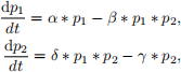
where α is the prey’s growth rate, β is the prey’s death rate, δ is the predator’s growth rate and γ is the predator’s death rate.

We want to model the population of snow hares (p1 ) and Canadian lynxes (p2 ).

Assume:

.  the population at is 100 hares and lynxes

.  all rates are constant

.  no other factors influence population size

Your final script should:

.  implement the predator-prey model with alpha = 0.48, β = 0.025, γ = 0.68 and δ = 0.02.

.  solve the system of differential equations at all timepoints in tYears using ode45 and the initial populations provided in p0  = [100, 5].

.  assign the resulting population estimates to a 2-column matrix named ppPop.  Prey should be in the

first column and predator in the second.

Answer: