Hello, dear friend, you can consult us at any time if you have any questions, add WeChat: daixieit

COMP5310 Principles of Data Science

Assignment 1 EXAMPLE REPORT

Problem

The History of Baseball data set has a comprehensive range of United States Major League Baseball player, team and other statistics spanning 145 years to the present day. Given its reasonably good quality and size, there are many different possible problems that could be explored. For this project, it was decided to focus primarily on understanding the relationship between individual player performance metrics, other player variables (particularly player salary and age), and overall team performance.

The challenge is to unlock the historical knowledge within this data set and gain insight into what factors are most important in determining baseball team outcomes. The problem to solve is that, given reliable personal attribute and performance data for baseball players, how can this information be used to: (a) make effective decisions regarding player selection, recruitment and retention, (b) assess team prospects based on the make-up of players, and (c) if possible, estimate the probabilities of future team success.

In the process, it is expected that the analysis would have application not only to Major League Baseball in the US, but also to other baseball leagues around the world. In addition, key learnings may be further generalisable to other similar elite sports.

Data

The data selected was the publicly available data set titled, “The History of Baseball”. It was downloaded from the Kaggle website located at the URL, https://www.kaggle.com/kaggle/the-history-of-baseball. The History of Baseball is based on Lahman’s Baseball database and consists of a compilation of recorded statistics for Major League Baseball in the United States between 1871 and 2015. It was assembled by the journalist Sean Lahman over a period from 1995 to present ('Sean Lahman' 2016).

Once extracted from the zip file, the folder contained separate files totalling 69MB in size. The actual dataset consisted of approximately 8.3 million data points across 25 separate tables stored as files in comma delimited value (csv) format. The master table comprises the list of all Major League players along with biographical and other data. The remaining tables provide information relating to player statistics (batting, pitching and fielding), plus information relating to the player salaries, teams, post-season statistics, and other details. The full list and explanation of the tables is provided in Appendix 1. More detailed breakdown of the fields within each table is summarised in the notes (Lahman 2015).

After reading supporting information (Kaggle 2016) as well as the notes from the data set author (Lahman 2015), some of the key tables were uploaded into a local installation of Jupyter notebook. For a few of the variables that were to be analysed graphically, the data was cleaned to remove nulls. However, no major transformation of the data was considered necessary. Preliminary analysis was then performed on the data (some samples of code used have been extracted and included in Appendix 5).

After importing a selection of the file data, the size of the more important tables was determined. Some statistics and histograms were then produced using Python code to get an understanding of the distribution of the data and summary information. Some examples of these histograms are shown in Appendix 2. A histogram of player size (using weight) was produced and appeared to show a normal distribution. After investigating a number of the physical characteristics and biographical details (such as college, birth state, etc.) of players, it was decided that these variables may not be very helpful in solving the main problem. Instead the focus shifted to other variables of interest.

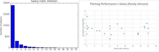
Figure 1 – (a) Histogram of player salary (USD, millions) and (b) scatter plot of pitching performance vs. salary.

Of particular interest was data pertaining to player attributes, performance and salary information (Figure 1 shows some initial data exploration results; more in Appendix 2). A histogram of salary was produced and appeared to show a power-law distribution (cf. Figure 1a); the exact relationship was not quantified. As is evident in Figure 1, a few players are receiving disproportionately high compensation compared to others and salary was considered worth investigating in depth (note salary was not normalised to compensate for price escalation over time).

In terms of individual player performance, histograms were created for select performance variables (RBI, SO). Some sample data was then analysed in Microsoft Excel (to allow easy filtering and manipulation of data from multiple tables) and examine the relationship between salary, age and a broader set of key performance indicators. Since salary data only goes back as far as 1985, more recent high performing players were analysed. In the case of a few players, they appear to have maintained high performance for a long period up to their late 30s, and it was considered interesting to find out the data regarding the age at which players peak.

The sample analysis revealed that it is not clear that salary increases always correlate well with performance improvement (cf. Figure 1b). Indeed, there may be very weak or no correlation at all with large salary increases mid career (observed for Darryl Strawberry for example). This requires more analysis across the players in the dataset to better understand the patterns. Some example comparisons of performance measures versus salary and age for sampled players are presented in Appendix 3.

Proposal

For stage 2 of the Project, the goal would be to understand, visualise and, where practicable, quantify the relationships between select individual performance measures (separately for batting, pitching and fielding measures) and other variables, as follows:

1. Individual player performance metrics profiles versus player age.

2. Changes in individual player performance metrics versus changes in salary.

3. Absolute measures of salary (adjusted for inflation) versus past player performance.

4. Depending on the outcomes above, it may be beneficial also to examine the relationship between salary and player public recognition (such as number of times selected for All-Stars).

5. Team performance (measured in end of season ranking and number of team wins) versus aggregate (mean, max etc.) individual player performance metrics.

The author's organisational structure for the data is designed around a relational database (Lahman 2015). Therefore, it is proposed that the analysis would be done by transferring the CSV files into PostgreSQL tables according to the schema provided with the data set. Specific queries would be performed using SQL statements, and then this data would be analysed in more detail and visualised using Python.

Performance measures would be prioritised. The focus would be on measures that are frequently used and initially based on measures identified in Appendix 4. If strong relationships are quantifiable, it is proposed to explore the feasibility of developing data models for predicting team / player performance and then test with the data set and assess the levels of confidence.

References

1. Kaggle 2016, History of Baseball, Kaggle, viewed 6 April 2016, https://www.kaggle.com/kaggle/the-history-of-baseball

2. Kaggle 2016, (Baseball dataset), Kaggle, https://www.kaggle.com/kaggle/the-history-of-baseball/downloads/baseball_2016-03-08-22-23-12.zip

3. 'Sabermetrics', Wikipedia, viewed 6 April 2016, https://en.wikipedia.org/wiki/Sabermetrics

4. 'Baseball Statistics', Wikipedia, viewed 6 April 2016, https://en.wikipedia.org/wiki/Baseball_statistics

5. Lahman, S 2016, Lahman’s Baseball Database, SeanLahman.com, http://www.seanlahman.com/baseball-archive/statistics/

6. Lahman, S 2015, The Lahman Baseball Database 2014 Version, http://seanlahman.com/files/database/readme2014.txt

7. 'Sean Lahman', Wikipedia, viewed 10 April 2016, https://en.wikipedia.org/wiki/Sean_Lahman

Appendices

1. Data table summary

2. Example aggregate data visualisation

3. Example sample player data visualisation

4. Example select performance measures

5. Samples of Python code

Appendix 1- Example aggregate data visualisation

The charts in the figures below show distribution of data for different variables relating to players.

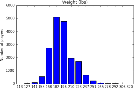
Figure 2.2 - Histogram showing distributions of player size (weight in lbs).

Appendix 3 - Example sample player data visualisation

The following charts show some example data of linking performance to various player variables. For example, below shows how select batting performance metrics changed with player age.

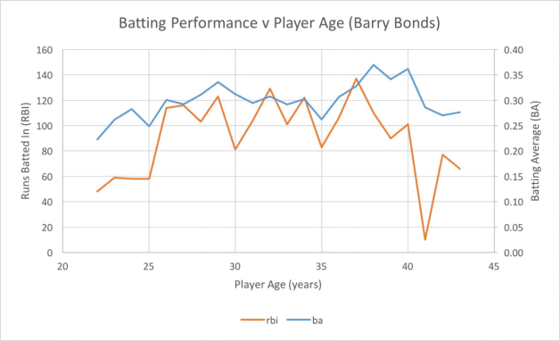
Figure 3.1 - Line chart showing sample comparison of batting performance measures versus player age