MATH3051 - COURSEWORK 1 AUTUMN SEMESTER 2023-2024
Hello, dear friend, you can consult us at any time if you have any questions, add WeChat: daixieit
SCHOOL OF MATHEMATICAL SCIENCES
AUTUMN SEMESTER 2023-2024
MATH3051 - COURSEWORK 1 — 20% —
Coursework 1 — Hand-in deadline: 13/Nov 8:00 GMT+1
Your report should be submitted electronically via the MATH3051 Moodle page by the deadline indicated there. Since this work is assessed, your submission must be entirely your own work (see the University’s policy on Academic Misconduct). Late submissions will be subject to a penalty of 5% of the maximum mark per working day.
Hand in a report and comment on all your results.
1. Consider the bivariate linear regression objective function, also called mean squared error. This function is expressed as

where  is a measurement for a given point
  while
while

is the linear two-variables function we aim to learn.
(a) Write down
i) the solution to the Least Squares Method
ii) the Gradient Method
iii) the Newton scaling in the Gradient Method
iv) the explicit form of the gradient and the Hessian.
(b) Import and normalize the data  from the file data.csv. Then, implement the gradient method with 100 iterations, initial guess x0 = (0,0,0), and stepsize (also known as learning rate) of 0.1, and print x100.
(c) Plot the bivariate regression along with the data.
(d) Run your code with a fixed number of iterations (100) and stepsizes 0.01,0.1,0.9, and plot the cost function (log scale) vs number of iterations (linear scale).
(e) Run your code with a fixed number of iterations (100) and stepsizes 1.9, 1.92, and plot the cost function (log scale) vs number of iterations (linear scale).
Table 1: Average High Temperatures at Nottingham
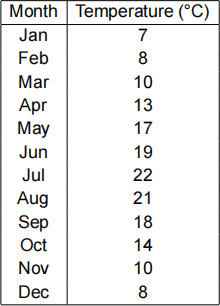
2. The average high temperatures from January to December at Nottingham Tk, k = 1, 2, … , 12 are given in Table 1.
The cyclical pattern of the temperatures suggests us to use a model in the form
f(t;x) = x1 sin (x2t + x3) + x4
to describe the relationship between the temperatures and their corresponding months, where the constant vector x = (x1,x2,x3,x4)T can be determined by solving the optimization problem
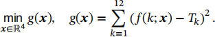
Use the Gauss-Newton method to solve the optimization problem.
(a) By looking at the properties of the function f, suggest reasonable values for x1, x2 and x4 in the starting point x0 of the iteration. Explain your suggestion based on the temperatures given in the table.
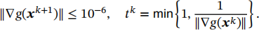
(b) Following the notations in the notes, write down J(xk) in the Gauss-Newton method explicitly. (c) Implement the Gauss-Newton method with x0 = (5, 1,0, 10) and a stopping rule of

(d) Implement a damped Gauss-Newton method with x0 = (5, 1,0, 10), stopping rule and stepsize given by
(e) Explain why are the big discrepancies in x1 and x3 in the answers of part (c) and (d) not surprising.
2023-11-02