CS 6210 Scientific Computing Assignment 3
Hello, dear friend, you can consult us at any time if you have any questions, add WeChat: daixieit
CS 6210 Scientific Computing
Assignment 3
Note: Please use Matlab, or a public domain approximation to it in this assignment. The code must compile on one of the lab machines with your instructions. Document your code thoroughly! As usual submit a clear report with your findings your name and the codes that you wrote and the results that they generated.
1. This is practical example of a large 1000x1000 linear system
The code to generate the matrix A of the system of equations and its righthand side b is given by
m = 1000;
for i=1:m
d(i) = 0.5 + sqrt(i);
end
A = diag(ones(m-100,1),-100) + diag(ones(m-1,1),-1) + diag(d) + ... diag(ones(m-1,1),1) + diag(ones(m-100,1),100);
b = ones(m,1);
Solve this system of equations by using the conjugate gradient method in its
original form and by using the diagonal form of the matrix A as a preconditioner.
( Note you will have to use the Magtlab documentation for the pcg code). An example of how to use this code iteration by iteration is given in the code
CGforHILB2iterbyiter.m on the canvas page. [20 Marks]
Code up the Gradient Descent method as given in the code SDescentHILB.m in the same code and show that it works. [15 Marks]
Run the three codes to get an accuracy of 1e-6 and compare their performance in
terms of iterations used. Move to an accuracy of 1e-16 and comment on the
performance of the methods. For about 8000 iterations the error of Gradient Descent is about 1e-23. Can you achieve the same accuracy with Conjugate Gradients?
Document your findings and produce graphs to show the residuals decrease for all the methods. [15 Marks]
2. (i) Modify the program that you wrote in the previous assignment for the “ Filip” data set that uses the Monomial Vandermode matrix approximation to produce a least squares approximation to work with this data set. In this case n=82 as there are 82 data points and m is the degree of the polynomial with m+1 terms. Use values of m equal to 9,11,13,15,17,19,21,23,25. Make use of the matlab QR or the Gramschmidt QR method given . Plot the values of the polynomial by evaluating the Monomial Vandemonde polynomial at (say) 1001 points and use plots in showing how the different polynomials behave. [10 marks]
Note that you do not have to plot every single case.
(c)In each case calculate the least squares error
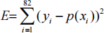 where yi are the data values at points xi and p(xi ) are the
calculated values of the polynomial.. [10 marks]
(d) I found that the QR method did not work well for larger values of m and the normal equations approach did. Use a linear scaling to put both x and y values in the range [-1,1] such as  . Repeat the experiments and show that
the QR results are better by producing before and after plots. [15 marks]
Compare the performance of the QR methods with solving the normal equations using your previous code [10 marks]
What to turn in
For these assignments, we expect both SOURCE CODE and a written REPORT be uploaded as a zip or tarball file to Canvas.
• Source code for all programs that you write, thoroughly documented.
o Include a README file describing how to compile and run your code.
• Your report should be in PDF format and should stand on its own.
o It should describe the methods used, explain your results and contain figures.
o It should also answer any questions asked above.
o It should cite any sources used for information, including source code.
o It should list all of your collaborators.
This homework is due on October 30th by 11:59 pm.
2023-10-28