Matrices, Vectors, and Differential Equations
Hello, dear friend, you can consult us at any time if you have any questions, add WeChat: daixieit
1. (20 pts) Suppose that A is a square, nonsingular, and non-symmetric matrix, b is an n-vector, and that you have called
L, U, p = cs111.LUfactor(A)
(using the routine from the lecture files). Now suppose you want to solve the system ATx = b (notAx = b) for x.
1.1. (10 pts) Show how to do this using calls to cs111.Lsolve() and cs111.Usolve(), without modify- ing either of those routines or calling cs111.LUfactor() again. You are allowed to transpose matrices L and U , that is, you may work with L.T and U.T. You may not call any of numpy’s built-in solvers (like npla.solve()).
1.2. (10 pts) Test your method in numpy on a randomly generated 5-by-5 matrix by proving that the relative residual norm jjb -AT xjj/jjbjj is essentially zero. Show your code and output in Jupyter.
2. (20 pts) Consider the linear system
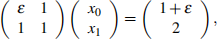
for some ε < 1. The exact solution is [x0 ;x1]T = [1; 1]T , independent of the value of ε .
For each value of ε = 10-4 ; 10-8 ; 10- 16 ; 10-20 , solve this system twice, using the routine cs111.LUsolve(), first with pivoting = True and then with pivoting = False. For each solution, print: the computed x; the error; and the relative residual norm returned by cs111.LUsolve(). Show your numpy code and its output. Comment on your results.
3. (60 pts) In class, we implemented the Jacobi iterative method using a matrix notation (x = (b - C @ x) / d), whereas we implemented the Gauss-Seidel iterative method using a component-by-component approach1 . The goal of this question is to implement the Jacobi iteration using the component-by-component approach. Recall that in Jacobi, we examine each ith equation in the systemAx = bin sequence (i.e., i = 0; 1; 2; :::; n- 1), and at the kth iteration, the unknown value x![]() k) is approximated as follows:
k) is approximated as follows:
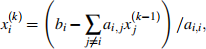
where a i;j is the entry at row i and column jin then-by-n matrix A, and bi is the ith element in b.
3.1. (30 pts) Write a Python function, named JacobiIterationSolve, that takes in a square matrix A, a vector b, a relative residual norm tolerance, and the maximum number of iterations, and implements the Jacobi method for solving the system Ax = b using a component-by-component approach. Your function should return the approximated solution x and a list of relative residual norms (one residual norm per iteration).
3.2. (30 pts) Test your implementation and compare it against the Gauss-Seidel iterative method, GSsolve, implemented in iterative.py. For this, suppose we set up the temperature problem for a 50-by-50 mesh (i.e, k = 50),with a fixed temperature of 1 on the top wall and 0 on the other walls. Plot the ap- proximated solution and print the number of iterations as well as the (last) relative residual norm, for each of your Jacobi implementation (JacobiIterationSolve) and Gauss-Seidel (GSsolve) meth- ods. To determine the number of iterations, use len( relRes ) - 1, where relRes isthe list of rela- tive residual norms returned by these functions. Take max_iters=10000 and tol=1e-8 as the default parameters in all methods. Also, plot the relative residual as a function of the number of iteration for both method on the same graph. Which method converges faster? Provide an intuitive reason as to why it converges faster.
2023-10-28
Introduction to the numerical algorithms that form the foundations of data science, machine learning, and computational science and engineering.