ENGG1001: Programming for Engineers — Semester 2, 2023 Assignment 2
Hello, dear friend, you can consult us at any time if you have any questions, add WeChat: daixieit
Assignment 2: Numerical Methods, Plotting and Object Orientated Programming in Python (25 Marks)
ENGG1001: Programming for Engineers — Semester 2, 2023
Due: Friday 20 October 2023 at 4:00pm
Introduction
The first task looks at some important features of Numpy arrays and their manipulation. The functions developed here should be very useful for practicing exam questions related to this, and assist in tasks 2 to 4, which continue our look at wind turbines (and their collection into windfarms) using authentic data gathered from AEMO (the Australian Energy Market Operator) and BoM (Bureau of Meteorology) .
The final tasks ( 5 to 9 ) explore the use of Object Oriented Programming in Python
Task 1:
Manipulation of numpy arrays is an important competency to be developed in ENGG1001 and a great skill to use for numerical programming and data analysis in Python. These manipulations find their way into the final exam, with typically 3–5 questions either directly or indirectly testing aspects of array manipulation (such as slicing, shaping, changing type, and operations with two arrays as variables) .
A nice array which helps frame examples of these manipulations is a sequential array, whose first term is 1 and each successive term by row then column is 1 greater than the previous one . For example, the 4 × 4 sequential array,
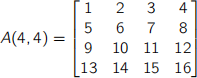
In python the corresponding array variable would be
1 np.array([[1,2,3,4],[5,6,7,8],[9,10,11,12],[13,14,15,16]]) # for integer type
2 np.array([[1.,2.,3.,4.],[5.,6.,7.,8.],...[13.,14.,15.,16.]]) # for float type.
A general sequential array is a sequential array, but with a starting value that may not equal 1. For example, a 2 × 2 matrix with a starting value of 5 would be represented as 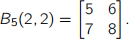
General sequential arrays with other dimensions also exist. Here are some examples:
0-dimensional array (effectively a scalar): B4() = 4
B = np . array([4])
1-dimensional array (a vector): B−10(3) =l−10 −9 −8]
B = np . array([- 10, -9, -8])
Write a function seq_array that receives a tuple (array shape) and an optional starting number s (default = 1.) which is either an integer or float, and returns the general sequential array with the shape provided and starting value s .
For example,
>>> array_shape = (4,)
>>> seq_array(array_shape)
array([1., 2., 3., 4.])
>>> array_shape = (3,2)
>>> starting_number = 5
>>> seq_array(array_shape,starting_number)
array([[ 5, 6],
[ 7, 8],
[ 9, 10]])
Task 2:
In Assignment 1 the first task involved writing a function determine_hub_speed(v_meas,
h_meas, h_hub, alpha) to correct wind speed at a measurement height to the wind turbine hub height.
def determine_hub_speed(v_meas, h_meas, h_hub, alpha):
"""Determine the wind speed at the hub, from ground data .
Parameters
v_meas: float
Wind speed measured at a height of h_meas h_meas: float
Height of at which the wind speed is measured h_hub: float
Height of the hub
alpha: float
Correlation coefficient
Returns
v_hub: float
The wind speed at the hub
"""
v_hub = v_meas * (h_hub / h_meas) ** alpha
return v_hub
For this task write a function determine_hub_speed_np(v_meas, h_meas, h_hub, alpha) to correct the wind speed for differences between velocity measurement height and hub height, using the speed and flexibilty associated with numpy arrays. Inputs to the function will be as follows: vmeas is a 1 dimensional numpy array, and hmeas , hubmeas, and alpha all float variables.
Output is the wind velocity at hub height, and will be a numpy array with the same shape as vmeas .
For example,
>>> v_meas = array([0.,2.,4.])
>>> h_meas = 10.
>>> hub_height = 80.
>>> alpha = 0.15
>>> determine_hub_speed_np(v_meas, h_meas, h_hub, alpha)
array([0., 2.73208051, 5.46416103])
Task 3:
Fluid Dynamics simulations (of which meteorological models are a subset) generally output fluid velocities in the directions of the co-ordinate system which the model uses. This is the case for the model used by the Bureau of Meteorology (BoM) from which we getting historical wind data.
In this model, hourly average predicted wind speeds at 10 m above ground in the u and v directions are output. The u direction is east-west (with wind direction to the east positive) and the v direction is north-south (with wind direction to the north positive) .
However, wind turbine power generated is a function of wind speed. For this task, write a python function which takes values of u and v wind components and outputs a tuple consisting of the wind speed and wind direction in degrees.
The convention for wind direction is that it is the direction which the wind comes from as measured using a compass. For example, wind with u = 1 m/s and v = 0 m/s has a wind speed of 1 m/s and direction 270 degrees (a westerly)
It is recommended that you use the arctan2 function in the numpy library to calculate wind directions.
A template for the function is provided below
def uv_to_speed_direction (u, v):
"""
Convert wind speeds from u and v components into speed and direction .
Parameters:
u (float): east-west component (towards east positive) m/s.
v (float): north-south component (towards north positive) m/s.
Returns:
speed_and_direction : A tuple containing wind speed (m/s) and wind <→ direction (in degrees, wind from the north = 0 or 360 degrees) .
"""
return speed_and_direction
Two examples follow .
![]()
>>> uv_to_speed_direction(1., 0.)
(1., 270.)
>>> uv_to_speed_direction(- 1 . , - 1.)
(1.4142135623730951, 45.0)
Task 4: Plotting power generation and wind speed
This task introduces some of the issues used when dealing with authentic data, in this case from wind speed data from BoM and windfarm power generation from NEM. The task focusses on the Capital windfarm, which lies just north of Canberra, and will be looking at January 2018 data. The following link1 gives some background information on the windfarm, including the type and number of turbines.
Information on the turbines, including a power curve (relationship between generation and wind speed at hub level) can be found here2. Power curve data (taken from the website) is in file power_curve. csv.
Wind speed data has been generated using the Barra R reanalysis data from BoM. The data is licenced under Creative Commons Attribution 4.0 International. Some processing of the data has been carried out, and the file capital_wind. csv contains hourly average windspeeds at the location of the windfarm over January 2018. The 3 columns of data are the time (in UTC which is effectively Greenwich Mean Time),u_ 10 (wind speed at 10 m height in u (Easterly) direction in m/s) and v_ 10 (wind speed at 10 m height in u (Easterly) direction in m/s) .
The final data file, capital_gen. csv, contains the average power generated for the Capital windfarm in January 2018, extracted from the NEM. The first column is time and the second is the power generation in MW.
Step 1. For this step write a function
generate_windfarm_power_curve(power_curve_filename, turbine_number) which reads the single turbine power curve and outputs a ‘Wind farm power curve’ of total wind farm power in MW versus wind speed. This will simply equal the single turbine power multiplied by the number of wind turbines in the wind farm, which is 67 in the case of the Capital wind farm .
The function’s output will be a numpy array with two columns and type float. The array’s first column will be the wind speed, and the second the wind farm power output expected at that speed.
Below shows the inputs needed to generate the Capital windfarm power curve, along with two properties of this output.
>>> output = generate_windfarm_power_curve( ' power_curve. csv ' ,67)
>>> output. shape
(26,2)
>>> output[-2:- 1]
array([[ 24 . , 140.7]])
Step 2. For this step write a function
This function will read in the time, wind speed and power generation data stored in the 2 file names provided, and output a tuple of three 1-dimensional numpy arrays.
The first member of the tuple is an array of times with datetime type with time in UTC. The datetime library has methods to convert date strings into datetime objects.
datetime. datetime.strptime(string, ' %d/%m/%Y %H:%M ' )) shows a possible syntax for such a conversion.
The second member is wind speed float type for hub height wind speed (m/s)
The final member is power float type containing values for power generation in MW
To generate the predicted wind farm power generation based on the predicted wind speed, you will need to first calculate the absolute wind speed based on its u and v components and correct for hub height ( use a hub height data of 80 m and alpha = 0.143 )
Below shows the inputs required to generate the time, wind speed and wind farm power for the Capital wind farm in January 2018, along with some properties of these files.
>>> (t_ar , w_ar , p_ar) =
‘→ generate_time_wind_power( ' capital_wind. csv ' , ' capital_gen. csv ' )
>>> t_ar. shape
(744,)
>>> t_ar[0]
datetime. datetime(2018, 1, 1, 0, 30)
>>> np . max(w_ar)
14.384398798026313
>>> np . max(p_ar)
132.201664
Step 3. For the final step in this task write a function
wind_farm_figure(windfarm_curve,times,wind,power) .
The input files will be the four numpy arrays containing the windfarm power curve, time, wind speed and power data which will have been generated earlier. The figure has no output but generates a single matplotlib figure.
This figure comprises 3 sub-plots
Subplot 1 - scatter plot of windfarm generation versus wind speed for January 2018 along with the windfarm power curve .
Subplot 2 - plot of power generated versus time for the 7 day period Jan 7 - Jan 14 .
Subplot 3 - plot of wind speed versus time for the same 7 day period.
Details on the exact layout of this figure are provided on Blackboard in a separate document.
An example of how this function may be called is shown below:
>>> capital_pc = generate_windfarm_power_curve( ' power_curve. csv ' ,67) >>> (t_ar , w_ar , p_ar) =
‘→ generate_time_wind_power( ' capital_wind. csv ' , ' capital_gen. csv ' )
>>> wind_farm_figure(capital_pc , t_ar , w_ar , p_ar)
In the remaining tasks (Tasks 5 -8), we will proceed to repeat the tasks from Assign- ment 1 using object oriented programming. Unless otherwise stated, the variable and the method/function definitions remain the same. These tasks will also require the same equations from Assignment 1.
Task 5:
Write a class called Site to store the data and functionality in relation to the wind turbine site. When creating a Site object, you will pass the site variables listed below. Your object needs to (privately) store these variables. Additionally, init method will initiate the measured speed v_meas, which will be set to 0 .
class Site :
def __init__ (self , alpha, rho, h_meas):
"""
Parameters
alpha: float
Correlation coefficient
h_meas: float
Height at which the wind speed is measured
rho: float
The air density
Returns
"""
def get_alpha(self):
""" Returns the correlation coefficient
Returns
float
Correlation coefficient
"""
def get_rho (self):
""" Returns the air density
Returns
float
The air density
"""
def get_height(self):
""" Returns the height of the measurement .
Returns
float
The height at which the wind speed is measured """
def get_meas_speed(self):
""" Returns the wind speed measurement .
Returns
float
The wind speed measurement
"""
float
The height at which the wind speed is measured """
def get_meas_speed(self):
""" Returns the wind speed measurement .
Returns
float
The wind speed measurement
"""
We can test this implementation at the console.
>>> site = Site(0.14, 1.225, 10)
>>> site . get_alpha()
0.14
>>> site . get_rho()
1.225
>>> site . get_height()
10
>>> site . get_meas_speed()
0
Task 6:
Add the following method to calculate the measured speed v_meas based on the speed measurements in the u and v directions. This is similar to Task 3; however, there is no need to calculate the direction of the wind speed.
...
def set_meas_speed(self , u, v):
""" Calculates and sets the measured speed.
Parameters
u: float
The wind speed measurement in the u direction (east-west) v: float
The wind speed measurement in the v direction (north-south)
Returns
"""
Again, we can implement this at the console.
>>> site = Site(0.14, 1.225, 10)
>>> site . set_meas_speed(0, 1)
>>> site . get_meas_speed()
1.0
>>> site . set_meas_speed(3, 4)
>>> site . get_meas_speed()
5.0
Task 7:
Write a class called Turbine to store data and functionality for wind turbines. When creating a Turbine object, you will pass the turbine variables listed below. Your object needs to (privately) store these variables. Additionally, __init__ method will initiate the hub speed v_hub, which will be set to 0 .
The method names with parameters and outputs are shown below. Note that cap_hub_speed is a new method that does not exist in Assignment 1. This method caps the hub speed v_hub at the rated speed.
class Turbine :
def __init__ (self , h_hub, r, omega, curve_coeffs, speeds):
"""
Parameters
h_hub: float
Height of the hub
r: float
The radius of the turbine blades
omega: float
omega
curve_coeffs: tuple
tuple of coefficients (a1, a2, ..., ak)
speeds: tuple
tuple of threshold speeds (cut-in, cut-out and rated speeds)
Returns
-------
"""
def get_hub_speed(self):
""" Returns the hub speed
Returns
-------
float
The hub speed measurement .
"""
def determine_hub_speed(self , site):
"""Determine the wind speed at the hub .
Parameters
site: Site object
An instance of the Site class
Returns
"""
def cap_hub_speed(self):
"""Caps the hub speed at rated speed
Parameters
Returns
"""
def determine_windpower(self , site):
"""Returns the wind power .
Parameters
site: Site object
An instance of the Site class
Returns
float:
The wind power
"""
def determine_mech_coef (self):
"""Returns the mech coefficient .
Parameters
Returns
float:
The mech coefficient
"""
def determine_mech_power (self , site):
"""Returns the mech power .
Parameters
site: Site object
An instance of the Site class
Returns
float:
The mech power
"""
The implementation is given in the console below.
>>> CURVE_COEFFS = (-2.579E-03, 2.311E-02, -2.155E-03, 3.703E-05, - 1.367E-06) >>> SPEEDS = (2, 15, 12)
>>> site = Site(0.14, 1.225, 10)
>>> turbine = Turbine(60, 40, 2.11, CURVE_COEFFS, SPEEDS)
>>> site . set_meas_speed(4,6)
>>> turbine . determine_hub_speed(site)
>>> turbine . get_hub_speed()
9.267078606531117
>>> turbine . determine_windpower(site)
2450.2166629351327
>>> turbine . determine_mech_coef()
0.4345560922031839
>>> turbine . determine_mech_power(site)
1064.7565780962173
Task 8:
Write a function named determine_total_energy that reads the hourly wind speed measurements from a csv file (e.g., capital_wind. csv from Task 4) and calculates the total energy with a given turbine and site over the observation time interval. You can assume that the conversion from mechanical power in the turbine to electrical power is 90% efficient. A sample usage of the function is given below .
>>> CURVE_COEFFS = (-2.579E-03, +2.311E-02, -2.155E-03, +3.703E-05, - 1.367E-06) >>> SPEEDS = (7.5, 17, 12)
>>> turbine = Turbine(60, 40, 2.11, CURVE_COEFFS, SPEEDS)
>>> site = Site(0.14, 1.225, 10)
>>> filename = "capital_wind. csv"
>>> determine_total_energy(turbine, site, filename)
51461.61794429864
Task 9:
This task involves creating a table which prints out the total energy generated for the given site scenario and the various potential turbine options. To create this table you need to write a function, print_table , which takes in turbine_parameters (a tuple of tuples), site_parameters (a tuple), separator (string) and filename (string) .
A example of the values in parameters is given in the tables below .
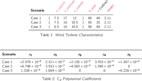
The function, print_table(turbine_parameters, site_parameters, separator, filename), does not return anything – it simply prints out the table.
A sample usage of the function is given bellow .
>>> turbine_parameters = (
(60, 40, 2.11, (-2.579E-03, +2.311E-02, -2.155E-03, +3.703E-05, -1.367E-06), <→ (7.5, 17, 12)),
(55, 35, 2.11, (-6.798E-03, +3.552E-02, -4.583E-03, +1.395E-04), (7.5, 16, <→ 10.5)),
(50, 40, 2.11, (+1.338E-03, +1.604E-02, 0.0E-00, 0.0E-00, -6.220E-06), <→ (6.5, 16, 10.5))
)
>>> site_parameters = (0.14, 1.225, 10)
>>> filename = "capital_wind. csv"
>>> print_table(turbine_parameters, site_parameters, ' * ' , filename)
*****************************************************
* Case number * Total energy (kW) * *****************************************************
* 1 * 51461.62 *
* 2 * 36913.49 *
* 3 * 136881.33 * *****************************************************
Writing your code
You must download the file, a2. py, from Blackboard, and write your code in that file. When you submit your assignment to Gradescope you must submit only one file and it must be called a2.py. Do not submit any other files or it can disrupt the automatic code testing program which will grade your assignments.
You must not import any external libraries other than the ones provided for you in the assignment folder.
Design
You are expected to use good programming practice in your code, and you must incorporate at least the functions described in the previous part of the assignment sheet.
Assignment Submission
You must submit your completed assignment to Gradescope. The only file you submit should be a single Python file called a2. py (use this name — all lower case) . This should be uploaded to Gradescope. You may submit your assignment multiple times before the deadline — only the last submission will be marked.
Late submission of the assignment will not be accepted. In the event of exceptional personal or medical circumstances that prevent you from handing in the assignment on time, you may submit a request for an extension. See the course profile for details on how to apply for an extension. Requests for extensions must be made according to the guidelines in the ECP.
Assessment and Marking Criteria (Total 15 marks)
Functionality Assessment (15 Marks)
The functionality will be marked out of 15. Your assignment will be put through a series of tests and your functionality mark will be proportional to the number of tests you pass. If, say, there are 25 functionality tests and you pass 20 of them, then your functionality mark will be 20/25 × 15. You will be given the functionality tests before the due date for the assignment so that you can gain a good idea of the correctness of your assignment yourself before submitting. You should, however, make sure that your program meets all the specifications given in the assignment. That will ensure that your code passes all the tests. Note that functionality tests are automated and so string outputs need to exactly match what is expected. Do not leave it until the last minute because it generally takes time to get your code to pass the tests.
Oral Presentation Assessment (5 Marks)
In the week following the assignment due date, students will be required to attend a short interview (of about 4 minutes) with a tutor in the Help Center. Students will be asked questions about their assignment code and they will be given a mark out of 5, based on the quality of their answers . Students will need to sign up for one of the interview time slots in Week 13. Details on how to sign up will follow .
2023-10-27
Numerical Methods, Plotting and Object Orientated Programming in Python