Investigating radioactivity using Maple

Requirement: Read the information below. Present your indings from Exercise  1  and  Exercise  2 in  a report with appropriate comments,  plots, equations, and other relevant outputs using Maple.  Once you have completed your report in Maple, you should convert the ile to a PDF and submit through the link in the ‘Assessment’ tab on Canvas. To convert your Maple worksheet (.mw ile) to a PDF select:

. File > Export As...  . Under the ‘Files of type’ drop-down select ‘.pdf’ .

Background:  For this task you will be required to use a mathematical model to make predictions about the levels of Radon in the environment. You will need to handle data measurements of Radon at given times using Maple to make appropriate predictions.

“Radon levels in the environment:  Radon is a radioactive gas, which decays with a half-life (T1/2) of only 3.8 days.  It originates from the rocks and soil and can be found everywhere in the environment.  Public Health England recommends that radon levels should be reduced in homes where the average is more than 200 becquerels per metre cubed (200Bq/m3 ).  1Bq = 1 decay per second.” Source: Public Health England.

Mathematical model:  Based on the work of Becquerel and Marie Curie (Nobel Prize winners).  Let N(t) be the number of radioactive particles at time t, then the rate at which the particles decay over time is proportional to the number of particles.  This can be expressed as dN/dt = -λN where λ is known as the decay constant. By separating the variable, this diferential equation can be solved giving N(t) = N(0)e-  t.

Errors:  Given n measurements (tk , yk ) of the numbers of particles yk , at time tk , for k = 1, ..., n, the model predicts the relationship y(t) = y0 e-  t. Ideally, yk  - y(tk ) is zero for  k  =  1, ..., n, but it is more likely to be very small.  Using a Least Square it, we deine the error function depending on N0  and λ ,

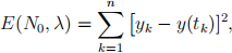
and ind the (optimal) values N0  and λ which minimise E.

Exercise 1:                                                                                [40 Marks]

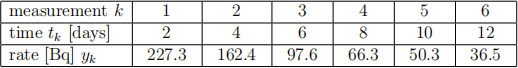
The radioactive decay rate of Radon in  1 m3   of  air was measured over  a period of 12 days. The results are:

The theory predicts the relation

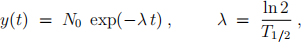
between the decay rate y and time t, where N0  is the initial decay rate - the object of interest - and the half-life is T1/2 .

(a)  Deine the Maple Array for y[1], . . . , y[6] and t[1], . . . , t[6] and assign the values from the above table.

(b) Deine the function E = E(λ, N0 ), using L for λ to avoid Greek letters and N0 for N0  to avoid subscripts, where

(c) Assign L(= λ) its known value speciied by 3.8 days half-life for the radon decay L   :=  log(2.)/3.8. Now use the plot command to show a graph of E as a function of N0  for 150  ≤   N0    ≤     400.  Convince yourself that this function has a minimum.

and hence solve the equation

What is your prediction for the initial decay rate N0  of the Radon in the container?