Hello, dear friend, you can consult us at any time if you have any questions, add WeChat: daixieit

MECH2700:  Computational  Engineering  &  Data  Analysis   (S2,  2023)

>  COVID:  Aerosol  Transport

Assignment  2:  Convection-Diffusion  Modelling

Aim

The aim of this assignment is to synthesise your understanding of parabolic and hyperbolic partial differential equations by developing a numerical scheme that models a physical process where both diffusion and convection are present. Your solutions are to be implemented in Python and formally documented in a report.

The Problem

COVID-19 has claimed more than 4.7 million lives worldwide [1]. In the early stages of the pandemic, it was widely believed that airborne transmission of the SARS-CoV-2 virus did not represent a signiicant risk [2]. However, mounting scientiic evidence (e.g. [3]) pointed to the reality of virus transmission by aerosols (e.g. diameter O (10 μm)) and droplets (e.g. diameter O (100 μm)) which are ejected from an infectious host via sneezing or coughing. The behaviour of these particles in the air (see Figure 1) is heavily dependent on their size, and yet the deinitions of both aerosols and droplets vary in the literature [4].

Figure 1: Computational luid dynamics simulation of aerosol and droplet trans- mission due to a cough, both (below) with and (above) without a mask [5].

With a limited number of assumptions, the distribution of virus-carrying aerosols and droplets in the air can be modelled as a combination of diffusive and convective processes. The unforced, two- dimensional convection-diffusion equation when convection only occurs in the x-direction is,

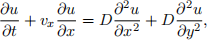
in which u is the particle number density (particles per cubic meter) and is a function of x, y and t, v x is a x-velocity that is only dependent on x, y and t, and D is a diffusion coeficient. The inluence of gravity would act tobias the diffusion towards the ground and manifests as a downwards drif ve- locity, while prevailing currents would transport the particles horizontally.

Consider the two-dimensional scenario shown in Figure 2, which is 10 mwide and 4 m high.  The person standing is carrying SARS-CoV-2 and shedding the virus. At some point in time, that person experiences a it of coughing which releases 104  particles into the air. It is assumed here that these particles are initially stationary and all located at the centre of the domain (i.e. location A), and that they are free to leave the domain from the sides and top. To model this, the appropriate boundary conditions are zero number density on the inlow boundary, x = 10 m,

u(10, y, t) = 0,

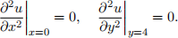
zero lux on the loor, y = 0 m,

and zero lux gradient on the top and lef boundaries

Your task is to predict the propagation of particles in the air and report on the particle number density at the location of the sitting person’s head (i.e. location B), in the time following their release.

Figure 2: The location of two people, one standing and one sitting, at the time of the coughing it.

Theirst step in the numerical solution method is to discretise the domain along its length and height into a grid of equally spaced nodes where spacing between nodes is Δx = Δy = 10/(nx - 1). nx is the number of nodes in the x-direction. The solution at a node located atx = iΔx, y = jΔyand t = mΔt

is denoted uj(i) .

Tasks

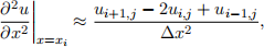
1.  Determine the discrete form of the convection-diffusion equation, at solution node (i, j).  To do this, approximate the second order space derivatives with the central difference expression (using u values at time step m) e.g.,

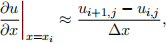
the irst order space derivative with the upwind difference expression (using u values at time step m),

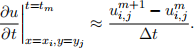
and the time derivative with a forward difference expression (equivalent to the forward Euler method for ODEs),

Present the discrete form of the governing equation for an arbitrary interior node i,j.  Given the known errors in the inite difference approximations used (derived in an earlier section of MECH2700), what is the order of accuracy of the discrete governing equation in space and time?

2.  Rearrange the discrete form of the governing equation from Task 1 into an update equation for an arbitrary internal node i, j (1    i    n x - 2, 1     j    ny  - 2) of the form,

Next, determine the update equations for on the boundaries with i = 0, j = 0, j = ny - 1 = jmax and i = nx  - 1  = imax.  To do this, you will need to utilize the discrete form of the boundary conditions,

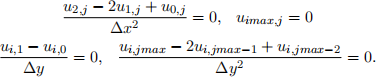
Note that the corner nodes do not inluence the rest of the solution for the numerical approach we are taking.

3. Write a Python function to determine a stable timestep for a numerical solution to this problem for arbitrary grid spacing Δx = Δy. This is to betaken to the following conservative combination of the hyperbolic and parabolic timestep expressions:

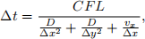
Here, conservatively take the Courant-Friedrichs-Lewy number to be CFL = 0.45. Note that when you ind a solution with different resolution, the stable timestep will change.

4. Write a Python function to advance the solution for by one time step that takes the current array of u, t, Δt and Δx as inputs.  Utilize this function within a Python program that advances the solution in the entire domain from the initial condition at t = 0 up to a maximum simulation time of t = tmax.  Record the full solution array every    5 s (to within Δt).  Also record the number density at the solution node nearest location B at every time step.  For the initial condition, take the number density at the node closest to location A to be u = 104/Δx2 , and zero elsewhere.

5. The diffusivity of the particles in the air is 0.01 m2 /s and the convection velocity is v x = -0.25 m/s. Assuming that the diffusion is unbiased (i.e. not inluenced by gravity), use your numerical scheme to predict the particle number density at location B for 20 seconds afer their release.  Generate contour plots of the particle number density distribution in the domain at 5 s, 10 s, 15 s and 20 s afer release. Also create a graph of the particle number density at location B with time. Does the count exceed a threshold value of 10 in this period?  How do your results change if the diffusion coeficient is halved to 0.005 m2 /s? Based on your results, would you anticipate a signiicant change in the exposure at location Bif gravity were accounted for by introducing a downward drif velocity of vy  = 0.01 m/s? Please explain your reasoning.

6.  Repeat the above calculation for at least one other choice of grid spacing.  Compare your results and comment on the grid-dependence of your numerical predictions. Hints: Be reasonable, here. If you try to run with a grid spacing of 1 mm you’re most likely going to have a bad time.  Also, include something in your code that tells you how far into your simulation you are.

The Report

Document your work in a formal report that includes, but is not necessarily limited to, the following: i.  Introduction: A brief description of the problem you have been asked to solve;

ii.  Methodology: The deinition of your approach to solving this problem, including all working and relevant assumptions;

iii.  Results: The appropriate presentation of results, which might include igures, graphs and tables;

iv.  Concluding Remarks: A critical discussion of your approach to the problem and your indings. At a minimum this should include comment on the stability, convergence, accuracy and compu- tational eficiency of your scheme.

Submission

Work individually or in groups of two for this assignment. Submit a single report for the group, de- tailing your analysis, code and results for Tasks 1 to 7.  This report should be brief but well struc- tured, so that the tutor can easily interpret your results.  Include your Python code and combine it alltogether into a single pdfile with a cover page that clearly tells us who you are. Scanned, hand- written documents with appropriate cut-and-paste items are perfectly acceptable, but plots should be computer-generated.

For assessment of your work, the tutors will be looking for answers to the following questions:

.  Have you done what the tasks require? Note that your report should be well structured and tidy so that the tutor can easily ind your answers. Having your plots correctly titled and axes labeled also helps a lot here.

. Are your answers accurate?

.  Is your code well-structured and clearly written, with suitable documentation comments? .  Does your code correspond to the results shown?